
If you want to know how to apply accounting number format in Excel, then you are in the right place!
In this article, we are going to show you some easy ways through which you can easily use the accounting number format in Excel.
Excel spreadsheets can be used for a variety of purposes, although they are most often utilized in the business and accounting industries. If you are working with Microsoft Excel for accounting reasons, you may want to consider using the accounting number format for the numbers you’re entering.
Similar to the Currency Format, there are other Accounting Formats that can be applied to numbers when they are required. It is important to note that, though, there is a distinction between using the Accounting format and using the Currency format. The Accounting format, for example, places the dollar sign at the extreme left end of the cell and shows zero as a dash.
Hence, there are so many ways to apply this format. Keep reading this post to know the details.
What Is the Accounting Number Format?
Numbers and other data can be formatted in Excel using a variety of options. Currency and Accounting number formats are both used for working with data connected to money and their associated accounts.
There are several similarities between these two presentation styles. At first sight, the accounting number format seems to be similar to the currency number format. There are, obviously, a few distinctions between the two methods.
These are the differences:
- Currency Sign: By selecting the appropriate cell or range of cells, you may display a number with the default currency sign to the very left.
- Zeros as Dashes: You can make your numbers display as dashes by using this format.
- Negatives in Parentheses: You can also show negative number values in the enclosure.
Excel’s standard accounting number format includes two decimal points, a thousands separator, and a dollar sign that can be locked to the extreme left side of the cell.
Difference between Currency and Accounting Format
At first sight, both the Currency and the Accounting Number formats seem to be almost identical in their structure and function. Although there are some similarities, there are also some important distinctions to be aware of.
Some of the differences are given below:
- The Currency format shows zero values as 0.00, but the Accounting number format shows zero values as a dash ‘-.’
- The Currency format shows the currency sign immediately next to the number, as opposed to the other formats. When using the Accounting number format, the currency sign is shown at the far left of the cell.
- Negative numbers are shown in the Currency format with a minus ‘-‘ sign, while negative numbers are displayed in the Accounting number format between brackets.
For the reasons stated above, numbers structured in the Accounting number format are more suitable for use in accounting applications.
How To Apply Accounting Number Format in Excel
Excel features a button on its ribbon that allows you to instantly utilize the accounting number format on your spreadsheets, which is convenient.
There are three different methods to use the Accounting number format for the numbers on your worksheet in Microsoft Excel:
- Make use of the Accounting Button.
- Utilizing the drop-down menu in the Number grouping.
- Make use of the Format Cells context menu.
Let’s take a closer look at each of the strategies listed one after another.
Using the Accounting Button to Apply Accounting Number Format in Excel
This is the fastest and most straightforward method of applying the accounting number format. Follow the procedures outlined below for using this technique:
- Choose the cells that need to be formatted.
- Choose the Home tab
- You will find the Accounting Number format shortcut button under the Number group.
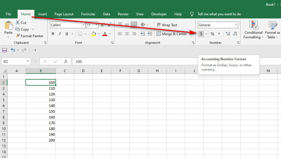
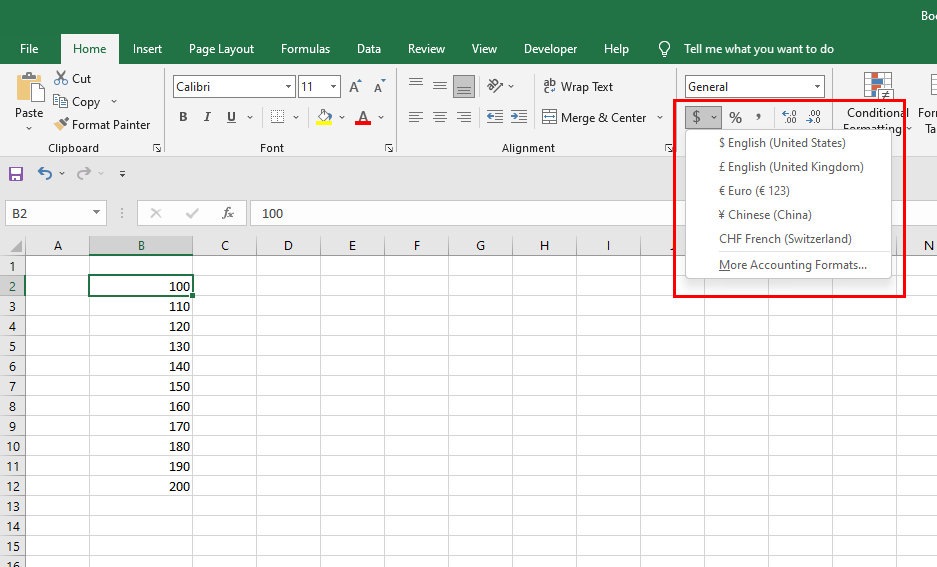
- If you wish to use the dollar symbol, click on the button. If you’d want to use a different currency sign, you can do so by clicking on the dropdown button next to the icon and selecting the currency you want from the selection list that pops up.
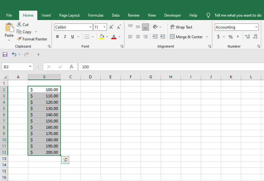
- The Accounting number format should now be applied to the cells that you specified. If you look to the far left of the chosen cells, you will discover your currency sign.
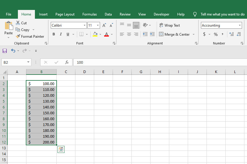
There are two decimal places in the number, which you will notice. You may adjust the number of decimal digits by clicking on the ‘Increase decimal’ or ‘Decrease decimal’ buttons, which will increase or decrease as needed. Separators in the thousands will also be noticeable. You will be unable to erase this separator off your number as long as you are using the Accounting number format.
Using the Drop-down Menu to Apply Accounting Number Format in Excel
You can find another easy way to use the accounting number format in Excel. Follow the steps below carefully to do that:
- Choose the cells that need to be formatted.
- Choose the Home tab
- You will find the format dropdown menu button (selected General) under the Number group.
- By selecting the menu option, you will be presented with a range of several formats that you may use to format the cells you have chosen.
- From the drop-down menu, choose the Accounting option to continue.
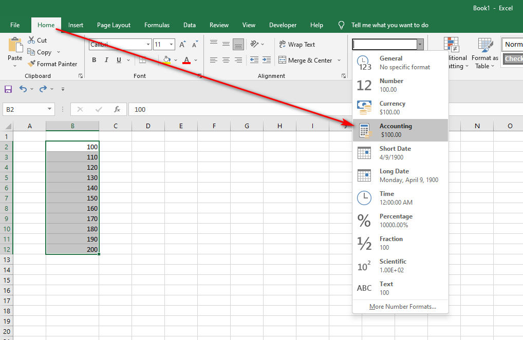
- Your chosen cells will now be structured in the Accounting number format, as seen in the example below. You’ll note that the currency sign is located at the extreme left of the cells you have picked.
The currency sign ($) may be replaced with some other currency symbol by selecting it from the dropdown menu that displays when you click on the arrow close to the dollar sign ($).
Using the Format Cells Context Meny to Apply Accounting Number Format
You may do any formatting actions on a cell or range of cells (such as alignment, font, margins, and so on) with the Format cells dialog box. It is a powerful dialog box that can be used in a variety of situations. To use the Format cells dialog box to utilize the Accounting number format for your cells, follow the procedures shown below.
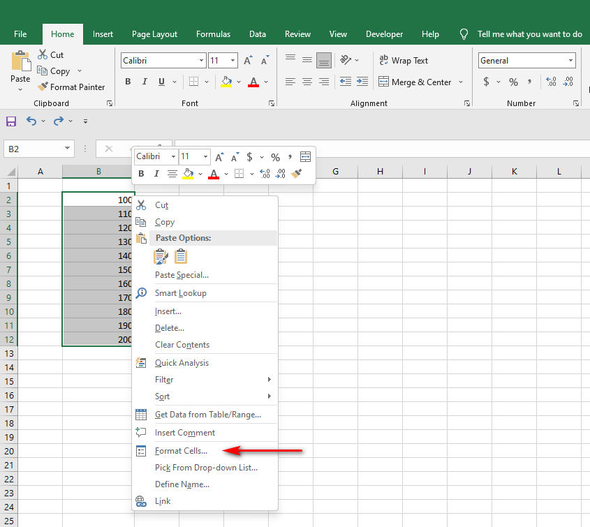
- Choose the cells that need to be formatted and Right-click on it.
- Make sure to pick Format cells from the contextual menu that opens.
- Click on the Number tab from the dialog box that opens.
- Select Accounting from below the Categories menu.
- This will show a preview on the top, allowing you to see how your number will appear when it has been formatted properly.
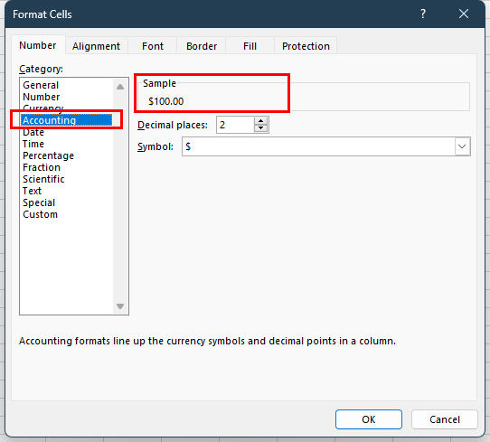
- In most cases, a dollar sign should be used to indicate the value. In order to use a different currency symbol, simply select it from the dropdown menu that appears when you click on the Symbol menu option next to it.
- In addition, you’ll see that the decimal point format is used. You may change the number of decimal places by clicking the arrow next to Decimal places.
- You may exit the Format cells dialog box by pressing OK.
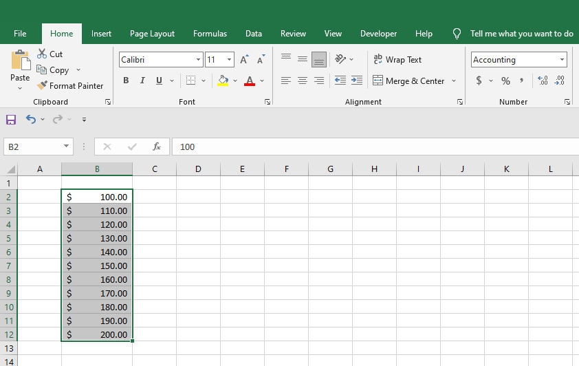
- The Accounting number format should now be applied to the cells you’ve chosen.
Conclusion
In Excel, using the accounting format is a snap. When putting together financial statements and balance sheets, as well as for other accounting-related tasks, the Accounting format might well be beneficial. We hope that this article has helped you understand how to apply the accounting number format in Excel.

