
One of the essential skills in Excel is the ability to skip cells when working with formulas. This skill is particularly important when dealing with data that is not consistent in length or when performing calculations on specific parts of a range of cells.
In this post, I will discuss how to skip rows in Excel. So, Let’s get started.

Understanding Cell References in Excel
Before I dive into the steps to skip blank cells in Excel using formulas, you must first understand cell references.
Cell references are used in Excel to refer to a specific cell or range of cells in a worksheet.
There are three types of cell references: relative, absolute, and mixed.
Relative cell references are the default type of reference in Excel. When a formula is copied to another cell, the relative reference changes based on the new location of the formula. For example, if you have a formula in cell A1 that refers to cell B1, and you copy the formula to cell A2, the reference to cell B1 will automatically change to B2.
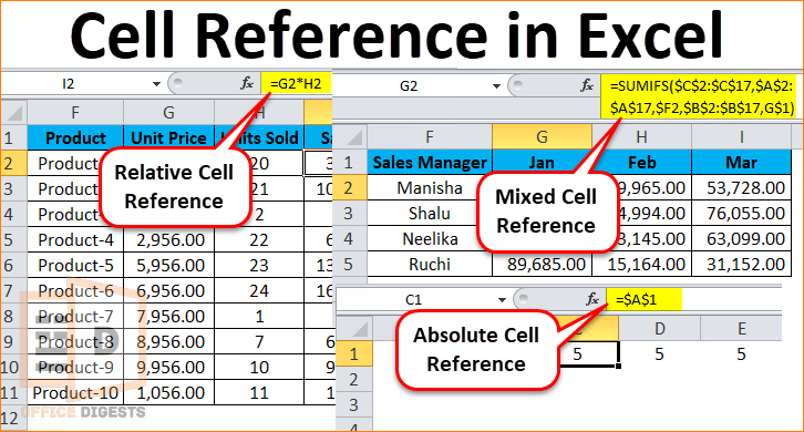
Absolute cell references, on the other hand, do not change when a formula is copied to another cell. To create an absolute reference in Excel, you use the dollar sign ($) before the column letter and/or row number. For example, if you have a formula in cell A1 that refers to cell $B$1, and you copy the formula to cell A2, the reference to cell $B$1 will remain the same.
Mixed cell references are a combination of relative and absolute references. You can use a mixed reference to lock either the row or column of a cell reference, while allowing the other part to change when the formula is copied to another cell.
Skipping Cells in Excel Formulas
Now that you understand cell references in Excel, let’s discuss how to exclude cells in formulas. There are two primary methods for skipping cells in Excel formulas: using relative references and using the SUM function.
So, here are the methods to skip cells in Excel using Formulas:
1. Use Relative References
Relative references can be used to skip cells in a formula. To skip cells using relative references, you simply add or subtract the number of cells you want to skip from the reference in the formula.
For example, if you have a range of cells from A1 to A10, and you want to sum only the values in cells A1, A3, A5, A7, and A9, you can use the following formula:
Alternatively, you can use a range reference with a step of 2 to skip every other cell in the range:
The colon (:) is used to define a range of cells, and the number after the colon represents the step size. In this case, I have specified a step of 2, which means that only every other cell in the range will be included in the sum.
2. Use the SUM Function
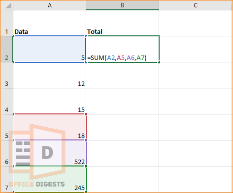
The SUM function can also be used to skip cells in a formula. To skip cells using the SUM function, you simply add or subtract the cells you want to skip as individual arguments to the function.
For example, if you have a range of cells from A1 to A10, and you want to sum only the values in cells A1, A3, A5, A7, and A9, you can use the following formula:
Alternatively, you can use the OFFSET function to specify the cells you want to include in the sum. The OFFSET function returns a reference to a range of cells that is a specified number of rows and columns from a starting point.
For example, to sum only the values in cells A1, A3, A5, A7, and A9 using the OFFSET function, you can use the following formula:
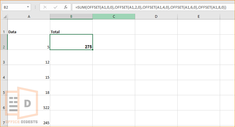
In this formula, the first argument for the OFFSET function is the starting cell (A1), the second argument is the number of rows to move (0), and the third argument is the number of columns to move (0).
The second argument for the next OFFSET function is 2, which means that the reference will be moved two rows down from the starting point (A1).
The third argument remains 0 because we are not moving horizontally. The same applies to the subsequent OFFSET functions, which move the reference four, six, and eight rows down from the starting point.
The OFFSET function is a powerful tool for skipping cells in Excel formulas because it allows you to specify the exact cells you want to include in a formula, regardless of their position in the worksheet.
How To Skip Cells When Dragging in Excel
Here are some additional tips and tricks for skipping cells in Excel formulas:
1. Use Named Ranges
Named ranges are a way to assign a name to a range of cells in Excel. When using formulas that skip cells, named ranges can make your formulas easier to read and understand.
To create a named range in Excel, select the range of cells you want to name, then click on the Name Box in the top-left corner of the worksheet and type a name for the range.
2. Use the IF Function
The IF function in Excel allows you to perform a logical test and return a value based on the result of the test.
When using the IF function with formulas that skip cells, you can use the logical test to check whether a cell should be included in the formula or skipped.
For example, the following formula will sum only the even-numbered cells in a range:
In this formula, the MOD function returns the remainder when each cell in the range is divided by 2. If the remainder is 0, it means the cell contains an even number, so the IF function returns the value in that cell.
If the remainder is 1, it means the cell contains an odd number, so the IF function returns 0. The SUM function then adds up all the values returned by the IF function.
3. Use the FILTER Function (Excel 365 only)
The FILTER function in Excel 365 allows you to filter a range of cells based on specific criteria. When using the FILTER function with formulas that skip cells, you can use the criteria to specify which cells to include in the formula.
For example, the following formula will sum only the values in cells A1, A3, A5, A7, and A9:
In this formula, the FILTER function returns only the values in the odd-numbered rows of the range A1:A10. The SUM function then adds up all the values returned by the FILTER function.
Final Words
Excluding blank cells in Excel is an essential skill that can help you work more efficiently with your data. Whether you use relative references, the SUM, OFFSET, the IF function, or the FILTER function, there are several ways to skip cells in Excel and perform calculations based on specific criteria.
By using these techniques, you can save time and streamline your data analysis processes.
Remember to always double-check your formulas and test them thoroughly before relying on them for important calculations.

