
As businesses and individuals, we often deal with large amounts of data that require sorting and filtering.
With that being said, Excel provides a powerful tool to manage such data, and creating a dynamic list based on criteria is a fundamental skill to master.
Organizing data is the first step towards making sense of it!
By defining a set of criteria, you can quickly filter data and update the list in real-time.
As an Excel power user, one of my daily activities is staying up-to-date with new Excel features.
So, in this tutorial, I’m going to show you how to create a dynamic list in Excel based on specific criteria and make the most out of this powerful feature.

How to Create Dynamic List in Excel Based on Criteria
Let’s look at a dataset where the total marks of each student of a class are given.
| Student ID | Name | Subject 1 | Subject 2 | Subject 3 | Total Marks |
| 1001 | Jessica Rose | 60 | 45 | 78 | 183 |
| 1002 | Misti Roy | 78 | 46 | 90 | 214 |
| 1003 | Nancy Irika | 82 | 59 | 75 | 216 |
| 1004 | Noman Akter | 54 | 76 | 80 | 210 |
| 1005 | Nidhika Khan | 74 | 91 | 67 | 232 |
| 1006 | Joy Rahman | 71 | 38 | 40 | 149 |
| 1007 | Tristan Nick | 59 | 42 | 85 | 186 |
| 1008 | Jona Ki | 89 | 64 | 94 | 247 |
| 1009 | Simran Ali | 60 | 90 | 28 | 178 |
My main objective is to create an active list from the above dataset using one or more criteria. So, Here are the methods to create dynamic lists in Excel:
1. Use The Combination of FILTER, COUNTA, and OFFSET Functions
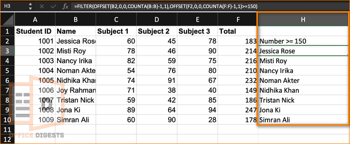
This method is applicable for Office 365 users only. Suppose I want to gather the results of students whose total marks are greater than or equal to 150. You can use other functions as well, but, for now, I am using the combination of Filter, CountA, and OFFSET functions.
The formula would be:
Detailed Breakdown of the Formula:
Let’s break down the formula and understand each part:
OFFSET(B2,0,0,COUNTA(B:B)-1,1): This part of the formula defines the range of data that needs to be filtered. It starts from cell B2 and goes down for a certain number of rows (determined by the number of non-empty cells in column B minus one) and across one column. Essentially, this creates a range of data from B2 to the last non-empty cell in column B.
OFFSET(F2,0,0,COUNTA(F:F)-1,1): This part of the formula determines the criterion for filtering. It starts from cell F2 and goes down for a certain number of rows (determined by the number of non-empty cells in column F minus one) and across one column. Essentially, this creates a range of data from F2 to the last non-empty cell in column F.
>=150: This is the criterion for filtering the data. The formula filters the data from the first range (B2 to the last non-empty cell in column B) based on the values in the second range (F2 to the last non-empty cell in column F). Only the rows that have a value greater than or equal to 150 in the second range are included in the filtered range.
FILTER(): This is the main function that filters the range of data based on the criterion. It returns only the rows from the first range that meet the filtering condition.
Final Result: See how Joy Rahman got eliminated in the final result. It’s because his total score was 149 which is below 150.
As we are discussing dynamic listing, try changing any value. The result will automatically change.
Now, what if you want to get the names of students who got total marks above 150 and also got above 50 marks in subject 2 (multiple criteria set).
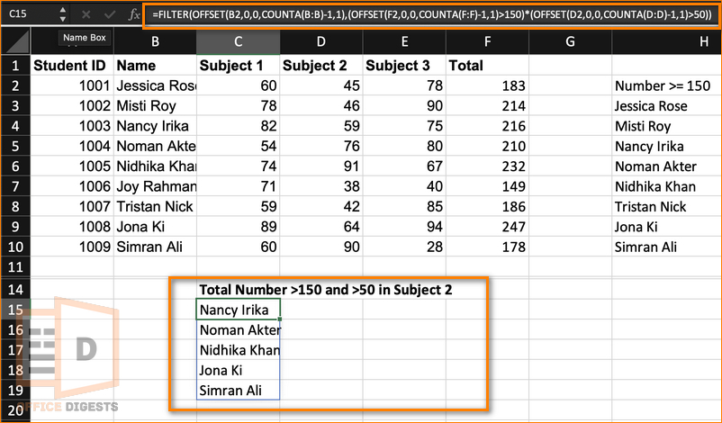
In that case, the formula will be:
Here, I just multiplied the formula *(OFFSET(D2,0,0,COUNTA(D:D)-1,1)>50)) to the initial one. You can set multiple criteria as your needs.
2. Create Dynamic lists in Excel with Data Validation
To create a dynamic drop-down list in excel with data validation tool, go through the following steps:
- Enter the list items in a separate range of cells. For example, enter the name of students in cells G1 through G10.
- Name the range of cells that contain the list items. To do this, select the cells containing the list items, click the Formulas tab on the ribbon, and then click Define Name in the “Defined Names” group. define-names-excel
- Click the Data tab on the ribbon by selecting a random empty cell and then click Data Validation in the Data Tools group.
- Select List from the Allow drop-down list. data-validation-excel
- Type the formula “=List1” (or whatever name you used to define the range of cells containing the list items) in the active cell.
- Click OK to close the Data Validation dialog box.
Now, when you click on the cell containing the dynamic list, a drop-down arrow will appear.
How to Create a Dynamic Unique List in Excel
The UNIQUE function in Excel is a dynamic array function that returns a list of unique values from a range or array of data. It eliminates duplicate values and displays only the extraordinary ones in the order in which they appear.
The syntax for the UNIQUE function is:
To create a dynamic list in Excel using the UNIQUE function, you can use the following steps:
- Create a table with your data and ensure that the headers are in row 1.
- Decide on the column that you want to create a unique list from.
- Enter the UNIQUE function in a separate cell and refer the range of data that you want to create a unique list from. For example, if you want to create a unique list from the Student ID column, enter =UNIQUE(A2:A10) where A2:A10 is the range of your data.
- Press Enter and the unique values will be displayed in the cell.
Note: To make the list dynamic, meaning that it updates automatically when new data is added to the table, you can use a named range with the UNIQUE function.
First, highlight the cell containing the UNIQUE function and go to the “Formulas” tab in the ribbon. Choose “Define Name” and give the named range a unique name.
In any other cell, enter the named range preceded by an equal sign. For example, if you named the range “IDList“, enter =IDList in the cell.
As I add new data to the table, the list will automatically update.
FAQ
What Is a Dynamic List in Excel?
A dynamic list in Excel is a list that is linked to a range of cells and automatically updates as the value of the cells alters. It is created using data validation, which is a feature in Excel that allows you to control what data can be entered in an active cell.
What is dynamic data in Excel?
Dynamic data in Excel refers to data that is automatically updated when the source data changes. I typically use it in scenarios where I need to display the most up-to-date information in your worksheets, dashboards, or reports.
Final Words
Exploration is the key!
The more you dig deep into the functions and formulas in Excel, the more creative you become. Just like making fire with a spark.
In this tutorial, I navigated you to the ways of creating a dynamic drop-down list. With this simple trick, you can now insert dynamic charts linked to a drop-down list in excel.

