
Navigating through a large Excel sheet can often feel like trying to find a needle in a haystack. Such a volume of information can be overwhelming, making it challenging to spot trends or crucial details.
That’s where alternating row colors come into play.
It’s like creating a visual roadmap for your data, making it remarkably easier to track, analyze, and comprehend. This feature has been a game-changer for Excel users worldwide.
In this guide, we will teach you how to use alternating row colors in excel so that you can turn your data from a sea of numbers into a visual masterpiece.

Alternating Row Colors in Excel
Alternating row colors, often known as zebra striping or banded rows, is a common practice in Excel. Most YouTube videos, along with some Excel gurus, will point you towards conditional formatting.
While you are busy using complex functions, or built-in equations, Excel offers a single solution.
In this section, we will guide you towards three methods to color rows alternatively.
Here are the ways to color every other row in Excel:
1. Format the Data as a Table
In our previous guide, we taught how to make Excel tables look good. You can create customized presets accordingly.
So, How to highlight every second row in Excel using Table?
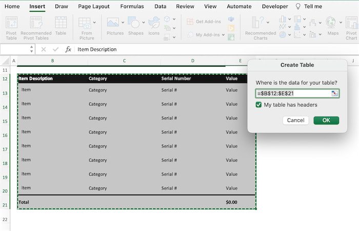
Select the range of cells you want to highlight and then go to the Insert Tab. Select the Table option. Verify the range of the data and click on the “My Table has Headers” option (if any). Click OK.
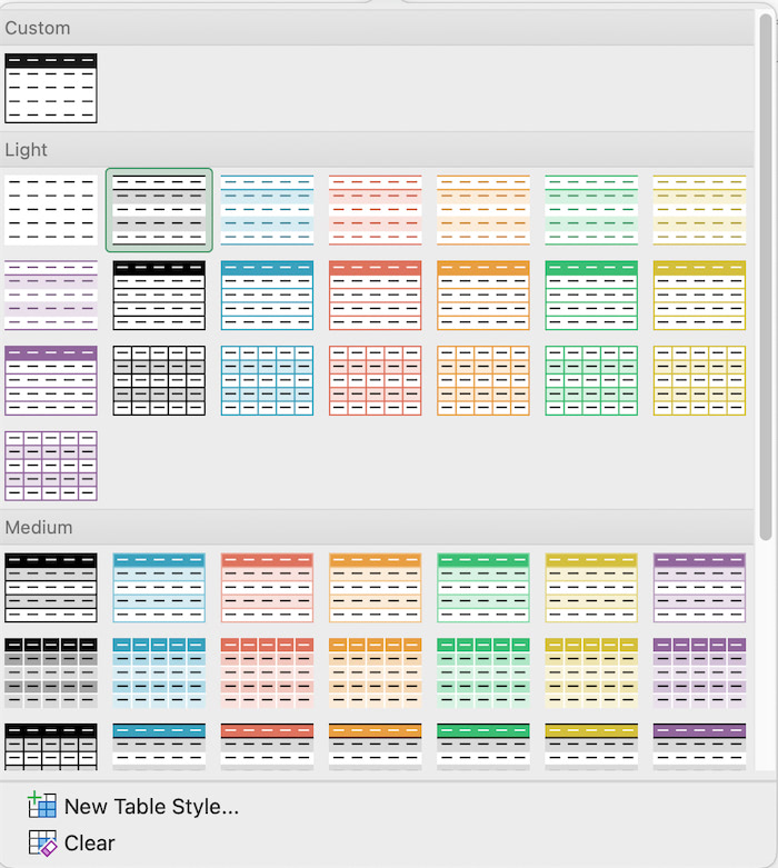
You can change the Table Design by clicking on the Table. Go to the Table Tab from the Ribbon bar and select any design you like.
There’s another method known as Conditional Formatting. Let’s get to know this process too in detail.
2. Use Conditional Formatting
Conditional formatting in Excel allows you to automatically apply formatting (like color changes) to cells based on specific conditions. This helps highlight important data, making it easier to spot trends or outliers.
The best thing about this feature is that you can choose from preset rules or create custom ones using formulas.
Conditional Formatting is dynamic, so if your data changes, the formatting adjusts accordingly.
So, here’s how you can utilize this feature to shade alternate rows or columns:
- Select the range of cells from the datasheet or press Ctrl+A to select the whole worksheet (if your dataset is large).
- Go to the Home Tab and Click on Conditional Formatting > New Rules.
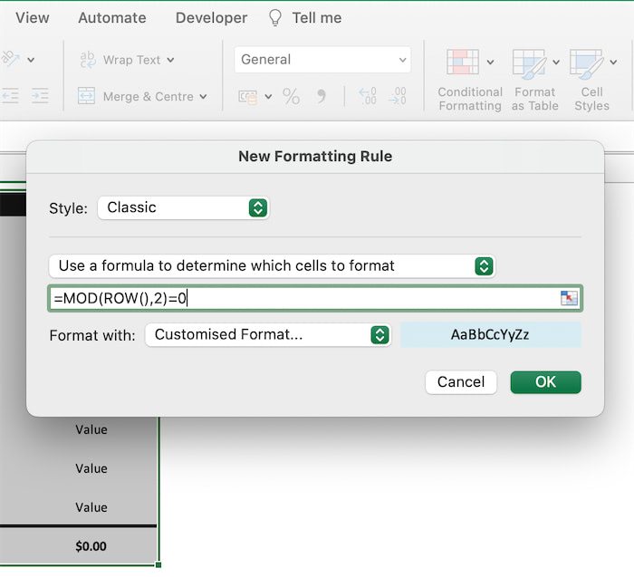
- Select the Classic Style (For MacOS), and select the option, ‘Use a Formula to determine which cells to format’.

- Type the formula =MOD(ROW(),2)=0 and select the ‘Customize Format’ button to apply preferable shades.
- Click OK.
Note: You can change the pattern or strip size of the banded rows using the Conditional Formatting feature.
Explanation of the formula:
The Excel formula =MOD(ROW(),2)=0 is used for distinguishing between even and odd row numbers within a spreadsheet.
When applied, it evaluates the remainder when the current row number is divided by 2. If the result is zero, indicating an even row, the formula returns a value of TRUE; otherwise, it returns FALSE for odd rows.
PRO TIP: If you want to shade alternate columns in Excel, then use the =MOD(COLUMN(),2)=0 Formula.
There’s one more method to add alternate row color in Excel. Let’s go through the method.
3. Apply A VBA Code
VBA codes in Excel is a shortcut method to get your job done in one-click. Think of it as a master button.
To add a VBA Code, you need to first enable VBA in Excel from the Developer’s Tab. After that, the option Visual Basic will be visible in the Ribbon bar.
Now, follow the steps below:
Open the Excel File and Press Alt+F11 to open the Visual Basic for Applications (VBA) editor. Click on Insert > Module. Paste the following code and Press F5 to Run the SubForm or module.
Code:
Sub AlternateRowColorBlue()
    Dim rng As Range
    Dim cell As Range
    Dim i As Integer
    ' Define the range where you want to apply alternating row colors
    Set rng = Range("B2:D10") ' Change this range as per your requirement
    ' Loop through each row in the range
    For Each cell In rng.Rows
        ' Check if the row number is even
        If cell.Row Mod 2 = 0 Then
            ' Set the row color (light blue in this example)
            cell.Interior.Color = RGB(173, 216, 230) ' Light Blue
        Else
            ' Set an alternate row color (white in this example)
            cell.Interior.Color = RGB(255, 255, 255) ' White
        End If
    Next cell
End Sub
You can change the RGB colors to add custom colors to your shading.
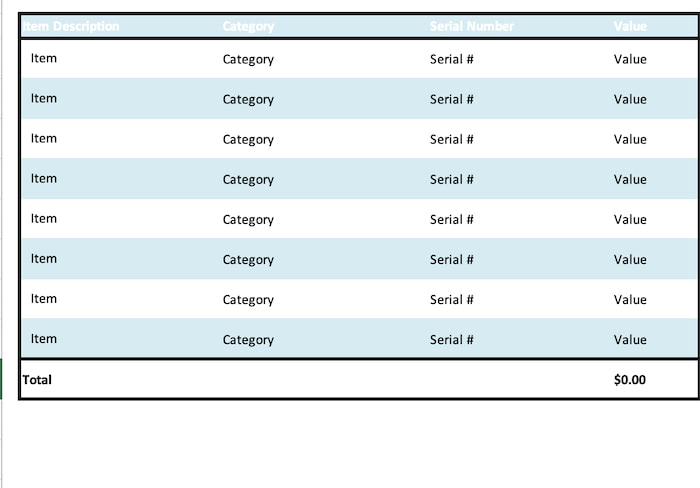
Result: The range of cells will be highlighted as light blue and white.
Conclusion
To transform dense data sets into visually organized information, there is no alternative option to shading. You can highlight rows and columns in Excel using the Table, Conditional Formatting, and even the VBA Code. For us, the default table design is the simplest and easiest workaround.

