CONCATENATE with VLOOKUP in Excel [With Examples]

Excel spreadsheets can be messy, with info scattered all over the place. That’s where CONCATENATE and VLOOKUP become the most iconic duo.

You use CONCATENATE to mush together different columns, creating a helper column. Then, with VLOOKUP, you can easily fetch data based on these combined values.

In this article, I’ll describe different ways of using CONCATENATE and VLOOKUP together in Excel with easy-to-understand examples.

Let’s begin!

Understanding the CONCATENATE Function

The CONCATENATE function in Excel combines text from multiple cells into one. It helps create a single text string by joining values. For example, =CONCATENATE(A1, ” “, B1) merges the contents of cells A1 and B1 with a space in between.

So, by using the CONCATENATE, or in short =CONCAT(), combine multiple text strings into one string. It takes two or more arguments, and you can concatenate up to 255 strings.

The syntax of the CONCATENATE functions is as follows:

The following table resembles the details of the arguments used in this formula:

Argument	Description
text1	The first text string or cell reference.
[text2]	This argument is optional. It represents additional text strings or cell references you want to concatenate.

Imagine you’re managing a sales spreadsheet in Excel, with separate columns for your clients’ First Name and Last Name.

However, to create a more polished and professional look in your communication, you decide to combine these columns into a single Full Name column. In that case, use the CONCATENATE function to achieve this seamlessly.

Simply enter the formula =CONCATENATE(A2, ” “, B2) in the adjacent cell of the first row of the “Full Name” column, assuming “First Name” is in column A and “Last Name” in column B. Excel will automatically concatenate the first and last names with a space in between.

As you drag this formula down to apply it to other rows, you’ll efficiently generate a complete list of full names without manually inputting each one.

VLOOKUP Function in Excel – At a Glance

The =VLOOKUP() is an excellent data-finding tool. In Microsoft Excel, it searches for a specified value in the first column of a range and returns a corresponding value from another column. It’s commonly used for data retrieval and lookup tasks to find information in large datasets.

Here’s the syntax of the VLOOKUP function:

The following table resembles the details of the arguments used in this formula:

Argument	Description
lookup_value	It is the value the function is supposed to search for in a table.
table_array	The range that contains the data.
col_index_num	The column number in the table from which to retrieve the value.
[range_lookup]	This argument is optional. Enter TRUE for an approximate match and FALSE for an exact match.

Suppose you’re managing a product inventory spreadsheet for an e-commerce business. Your sheet lists product IDs in one column and corresponding product names in another. To quickly retrieve product names based on their IDs, you can use the VLOOKUP function.

Let’s say you have an order list with product IDs, and you want to fill in the product names automatically.

Just apply =VLOOKUP() to search the product ID in the inventory sheet, and the function will return the associated product name.

Now that you know what VLOOKUP and CONCATENATE are and how to use them, let’s find out how to use the functions together.

How to Use VLOOKUP with CONCATENATE in Excel

Use the VLOOKUP function in combination with CONCATENATE to perform a lookup based on concatenated values.

Applying CONCATENATE allows you to merge two or more columns into a single cell. Subsequently, you can employ VLOOKUP to search for a specific concatenated value in a designated table array and retrieve corresponding information from another column.

This process is beneficial when dealing with composite keys or matching data based on a combination of multiple criteria.

Here’s how to use VLOOKUP with CONCATENATE in Excel:

1. Combine CONCAT with VLOOKUP

You can use multiple VLOOKUP functions to extract different information from a table and then concatenate the results in another cell.

Suppose we have an Excel dataset of employee information where column A contains the Employee ID, and columns B and C have the first and last names in cells A2:C6.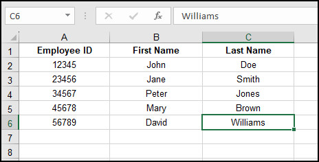

For this example, we’ll create a dropdown menu of Employee ID, and when you select an ID, you’ll get the employee’s full name in another cell.

To make the dropdown menu, first select the cell. Here, I’ve chosen D3. Now, go to the Data tab and select Data Validation from the Quick Access toolbar.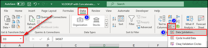

Choose List in the Allow field and select the Employee ID column in the Source field.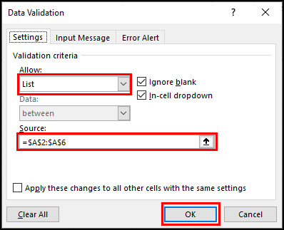

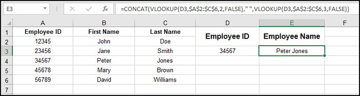
Then, select an empty cell, let’s say E3, and enter the following formula:

Here’s a breakdown of the code:

This part looks up the value in D3 in the range A2:C6 and retrieves the corresponding value from the second column (First Name).

This part looks up the same value in D3 in the range A2:C6 but retrieves the corresponding value from the third column (Last Name).

Finally, this part concatenates the results of the two VLOOKUP functions separated by a space.

2. Ampersand (&) to Concatenate with VLOOKUP

Let’s use the & (concatenate) and VLOOKUP functions together.

In this example, we’ll imagine a scenario where you have a list of products and their corresponding prices, and you want to create a new column that concatenates the product name and price.

Then, you’ll use VLOOKUP to find the price of a specific product based on a lookup value.

Assuming that you have a worksheet in Excel with two columns, where Column A has a product list from cell A2:A4, Column B consists of the price of the products from cell B2:B4.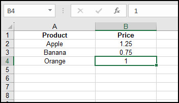

Now, let’s create a new column that concatenates the product name and price.

In cell C2, enter the formula:

This formula concatenates the product name in column A with the text ” – $” and the price in column B.

Drag the formula down for the other rows.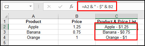

Now, let’s use VLOOKUP to find the price of a specific product.

In cell B10, enter the product you want to look up, for example, Banana.

In a cell where you want to display the result, let’s say B12, enter the following VLOOKUP formula:

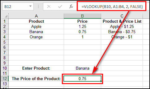
Here, B10 represents the lookup value of the product you want to find the price for. A1:B4 is the range of your dataset (product names and prices). 2 returns price is from the second column, and FALSE provides the exact match.

3. Create a VLOOKUP Function to Concatenate in Excel VBA

Utilizing the power of Visual Basic for Applications, you can construct custom VLOOKUP functions to enhance data manipulation capabilities. By combining =VLOOKUP() with VBA, you can seamlessly concatenate data from different columns based on specified lookup conditions.

Here are the steps to create a VLOOKUP to concatenate in Excel VBA:

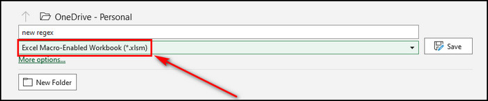
• Open Microsoft Excel and save the file as Excel Macro-Enabled Workbook (*.xlsm).
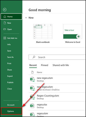
• Select File > Options.
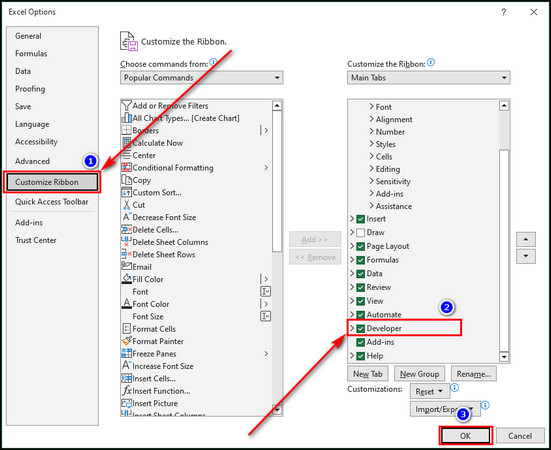
• Proceed to the Customize Ribbon tab, put a checkmark on Developer, and click OK.
• Move to the Developer tab and click on Visual Basic.
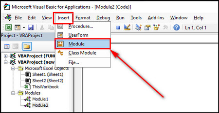
• Choose Insert > Module.
• Type in the following function in the module and save it:

Function CustomVLookup(lookupValue, lookupRange As Range, columnIndex As Long) As String
    Dim cell As Range
    Dim result As String
    For Each cell In lookupRange
        If cell.Value = lookupValue Then result = result & " " & cell.Offset(0, columnIndex - 1).Value
    Next cell
    CustomVLookup = Trim(result)
End Function

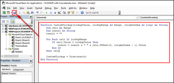
This Visual Basic for Applications code defines a custom function called CustomVLookup. This function performs a lookup operation similar to the Excel VLOOKUP function but is implemented in VBA code.

Now, suppose we have an Excel dataset with four columns where column A & B contains the first & last names, and columns C holds the departments’ names, and column D is the helper column in cells A2:D6. 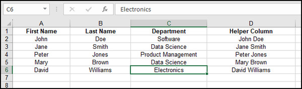In this example, we’ll enter a department name in an empty cell, let’s say in cell B10.

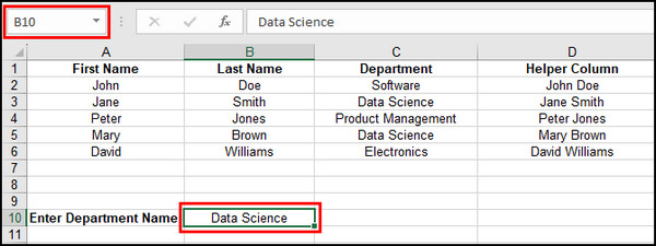
Enter the following formula in an empty cell:

The cell will display all the user names associated with the chosen department.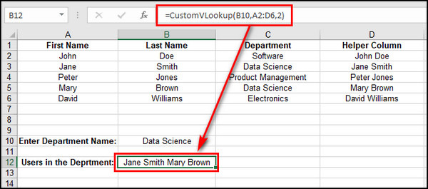

Final Words

As you can see, the combination of CONCATENATE and VLOOKUP in Excel is a powerful and efficient tool for data manipulation and analysis. By merging data from multiple sources with CONCATENATE and using VLOOKUP to retrieve relevant information, you can simplify your work and gain valuable insights.