Count Unique and Distinct Values in Excel [With Examples]

If you ever need to count with exceptions, and especially if these exceptions are more than one thing, which is normally the case in real life, then the countifs function is for you.

While dealing with a large dataset, we come across two different values, Unique and Distinct Values. Unique values appear once in the list, whereas distinct values are unique values + first occurrences of duplicate values (More on that later).

In this post, we will get to know how to count unique values in Excel with formulas alongside getting an automatic count of distinct values in a pivot table.

How To Use COUNTIFS Function to Count Unique Values in Excel

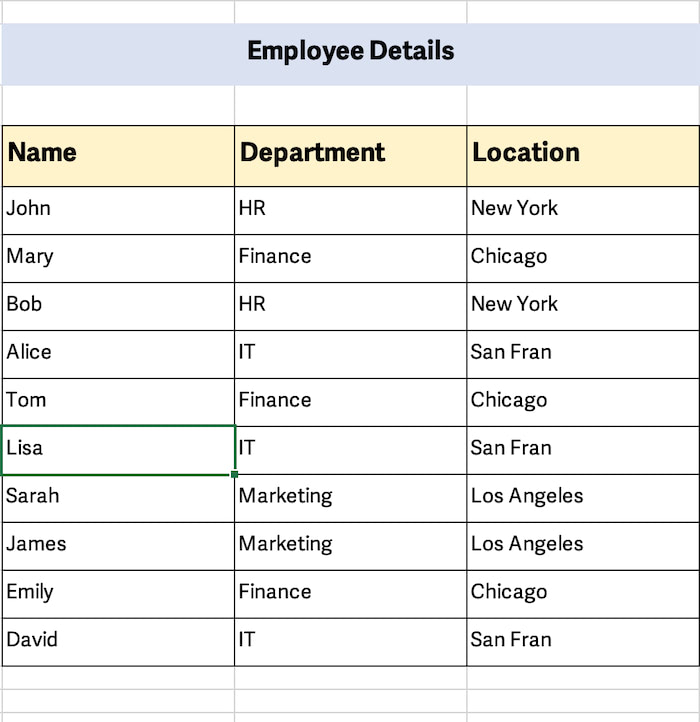
As an example, we will be using a record containing Employee Details (their name, designation, and location). The dataset contains both unique and distinct values for easy understanding.

Note that this example is a basic one. In real life, you will face complex problems. But rest assured, you will learn all the basics regarding the COUNTIF Function to deal with those situations.

Let’s get to know a combination of a few formulas to count unique values of different types.

Get Hands-On: Download the Practice Workbook and Work Along with the Steps

You can click below to download the practice workbook and follow along with the step-by-step instructions.

Download COUNTIFS Distinct and Unique Values in Excel.xlsx

 

Count Unique Text Values in a Column

First, let’s define the two terms (unique and distinct values) and get to know how to find them using formulas.

Unique Values: These types of values appear only once in a range of data.

Distinct Values: These types of values contain both unique and duplicate values. But, the duplicate value will appear once.

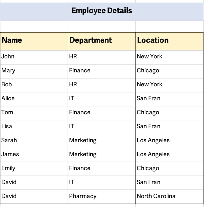
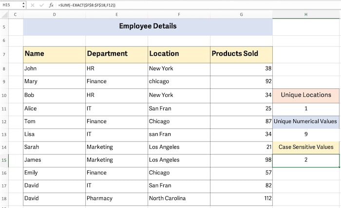
Look at the image below. Consider only the Department column. Can you distinguish between the two types?

Unique value: Pharmacy

Distinct value: Pharmacy, HR, Finance, Marketing, IT.

We will be using a combination of functions (COUNTIFS, SUM, IF or ISTEXT) to calculate individual text values. Only COUNTIFS is an array formula here. Check out our guide on how to create a table array argument in Excel if you are unknown to this topic.

Syntax of COUNTIFS:

The formula we will be using for our dataset will be for calculating the unique location in the F column.

We will use-

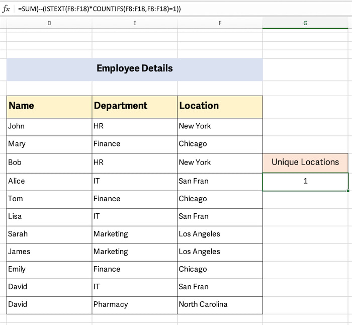
Click on any cell and use the above-mentioned formula, and press Ctrl+Shift+Enter for Excel to return a result.

Explanation of the formula:

The formula counts the number of unique text values in the range F8:F18. It does this by first checking if each cell contains text, then counting how many times each value appears, and finally summing up the values where the count is equal to 1, indicating uniqueness.

Note: The double unary operator (–) is used to convert the array of 0s and 1s into a numeric array where 0 remains 0, and 1 remains 1.

Count Unique Numerical Values

We have to keep two things in mind.

1. Similar numbers won’t be counted while counting unique values. Suppose your data contains 11 numbers, out of which two are the same. So, your total count will be 9.
2. Excel considers date and time format as numerical. So, these values will be counted.

In this section, we will use the ISNUMBER Function instead of the ISTEXT. We enlarged our dataset and added a column (Products Sold) to the list. So, our formula will be:

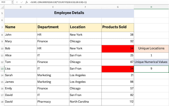
This formula works similarly to the previous one. It checks if each cell in the range G8 to G18 contains a numeric value and counts how many times each value appears in the range.

You can use the COUNTIF Function as well, since there is only one condition.

Count Case-Sensitive Unique Values Using COUNTIFS

In Excel, case-sensitive data refers to information where the distinction between uppercase (capital) and lowercase (small) letters is significant. For example, in a case-sensitive context:

“Chicago” and “chicago” would be treated as two distinct entries.

Note: COUNTIFS function returns in case-insensitive matches. We have to combine the EXACT function along with the SUM function.

The EXACT function in Excel is used to compare two text strings and determine if they are exactly identical, including being case-sensitive.

Suppose we want to find out how many times the word “Chicago” was used in our dataset. We have 1 lowercase chicago word. Notice that the word will be eliminated in the final result.

So, our formula will be:

Count Unique Values With Multiple Criteria

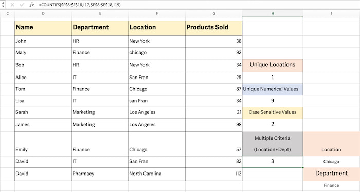
We will now use the COUNTIFS function implementing multiple criteria. Our criteria is to find the number of employees who are from Chicago designated as Finance Officers.

By considering the two criteria, our formula stands-

After pressing Enter, Excel returns a result = 3. But, remember that, even if your data contains case-sensitive values, it won’t be counted. You have to use the EXACT Function.

Use UNIQUE And ROWS Function To Count Unique Values

In this section, we will use the combination of IF, ISTEXT, ROWS, UNIQUE, and COUNTA functions.

Select the range of cells and use the formula =COUNTA(UNIQUE(range)). Now, to find unique texts only, use the formula =ROWS(UNIQUE(IF(ISTEXT(range,range)))-1. Press Ctrl+Shift+Enter to return the result.

How To Count Distinct Values in Excel Using COUNTIFS

To work with distinct values in Excel, you can use functions like COUNTIF, COUNTIFS, SUM, and SUMPRODUCT in combination with array formulas. These functions allow you to perform calculations or operations only on the unique values in a dataset.

For example, if you want to count the distinct values in a range, you can use the COUNTIF function with a criterion that checks for uniqueness. If you want to perform more complex operations based on multiple conditions, you might use COUNTIFS.

Note: Excel doesn’t have a dedicated built-in function solely for counting distinct values.

In this section, we will be using two general formulas to count distinct values in Excel. The formulas are in a combination form (using SUM and SUMPRODUCT).

Stick with us till the end, because we will be showing you a built-in alternative method to find out the number of distinct values.

Let’s organize our dataset and find out the number of distinct employees, their departments, and salaries individually.

To find the exact number of departments, we can’t use the ISNUMBER or ISTEXT Function because it will count unique values if done so. For this reason, we will use the SUM or SUMPRODUCT Function. Our formula will be:

Explanation of the formula:
This formula first uses the COUNTIFS function. COUNTIFS counts the number of cells in a range that meet multiple criteria. Here, the range is F7:F19. The criteria is specified as F7:F19, F7:F19, which means it is comparing each cell in the range to the entire range itself.

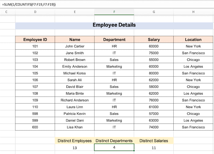
After pressing Ctrl+Shift+Enter, the result of COUNTIFS(F7:F19, F7:F19) is an array of counts, where each count corresponds to the number of times a particular value occurs in the range.

To get the distinct count, we take the reciprocal of each count using 1/, effectively converting counts to fractions.

Finally, the SUM function is used to add up all these fractions, which gives the total number of distinct values.

So, how Excel calculates the Distinct values?

Suppose we have a list of fruits:

• Apple
• Banana
• Apple
• Orange
• Banana
• Apple
• Mango
• Orange
• Banana

Step 1: Count How Many Times Each Value Appears

Using the COUNTIF function, we count the occurrences of each fruit:

Apple: 3 times

Banana: 3 times

Orange: 2 times

Mango: 1 time

Step 2: Convert Duplicates into Fractions

Now, we turn these counts into fractions. If a value appears 2 times, it generates 2 items in the array with a value of 0.5 (1/2 = 0.5). If a value appears 3 times, it produces 3 items in the array with a value of approximately 0.333 (1/3 ≈ 0.333).

The array becomes:

Apple: 0.333, 0.333, 0.333

Banana: 0.333, 0.333, 0.333

Orange: 0.5, 0.5

Mango: 1

Step 3: Apply the SUM Function

When we use the SUM function on these fractions, the sum of all fractional numbers for each individual item always yields 1, no matter how many occurrences of that item exist in the list.

Apple: 1

Banana: 1

Orange: 1

Mango: 1

Step 4: Calculate Total Different Values

Since all unique values appear in the array as 1 (1/1 = 1), the final result returned by the formula is the total number of all different values in the list.

Final Result: Here, there are 4 different fruits- Apple, Banana, Orange, and Mango.

Now, let’s look at some real-life complex scenarios where you might want to apply the COUNTIFS Function.

Count Distinct Values Ignoring Empty Cells

Zero (0) is also a number. So, when you have a dataset containing multiple empty cells, you might want to ignore them. But how?

You have to use the IF Function in addition to the COUNTIFS. So, our formula will be:

Explanation of the Formula:

This Excel formula is used to determine the total count of distinct values within a specified range, which in this case is H7:H19. The formula begins by evaluating each cell in the range to check if it is not empty.

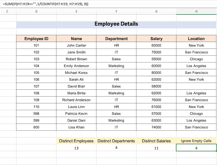
If a cell is not empty, it proceeds to calculate the reciprocal of the count of that specific value in the range. This step is crucial as it converts the counts into fractions, making it easier to identify unique occurrences.

If a cell is empty, the formula returns a value of 0. Subsequently; the formula adds up all these fractional values using the SUM function.

The final result provides the total count of distinct values in the specified range, reflecting the number of unique items present in H7:H19.

Other Necessary Examples

We will now show the criteria and formula of each criteria inside a table so that you can easily catch the difference between calculating a unique value and a distinct value.

Criteria	Formula
Count distinct text values	=SUM(IF(ISTEXT(range),1/COUNTIF(range, range),””))
Count Distinct Numbers	=SUM(IF(ISNUMBER(range),1/COUNTIF(range, range),””))
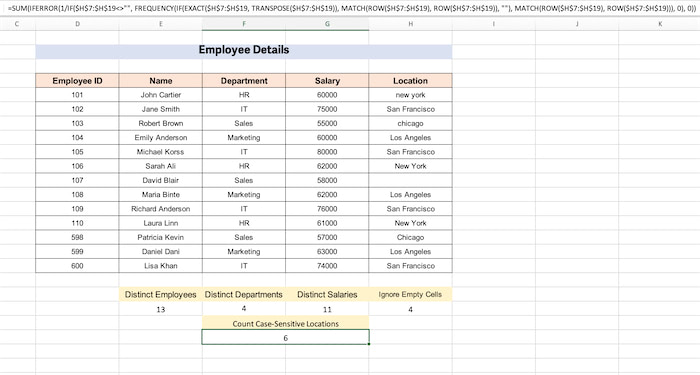
Count case-sensitive distinct values	=SUM(IFERROR(1/IF($H$7:$H$19<>””, FREQUENCY(IF(EXACT($H$7:$H$19, TRANSPOSE($H$7:$H$19)), MATCH(ROW($H$7:$H$19), ROW($H$7:$H$19)), “”), MATCH(ROW($H$7:$H$19), ROW($H$7:$H$19))), 0), 0))

Count Distinct Values Using Advanced Filter (Alternative Method)

Excel has an advanced filter option. It helps to separate distinct records only to a preferable location.

Here are the steps to use the advanced filter function to count distinct values in Excel:

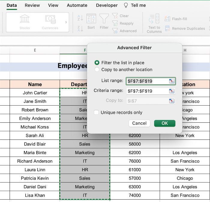
1. Select the range of cells and go to the Data Tab.
2. Click on the Advanced Filter options.
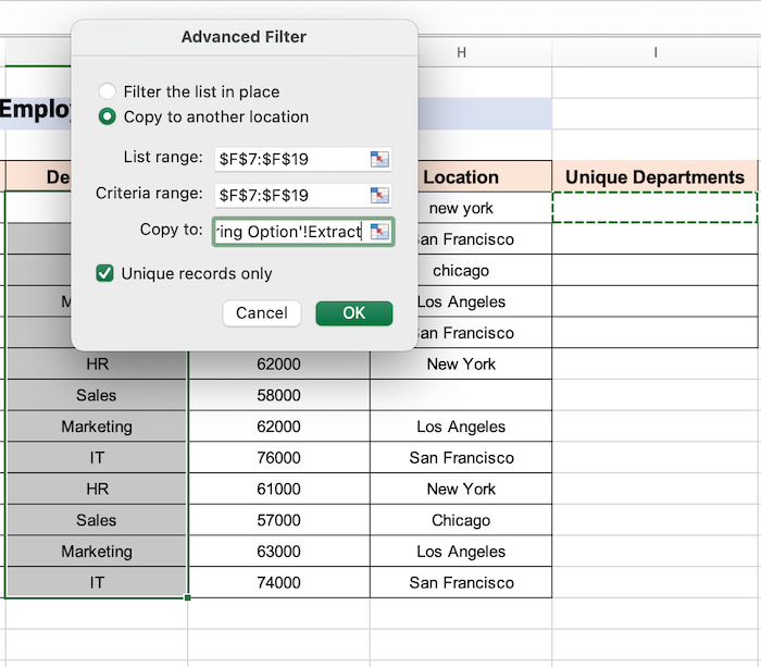
3. Select the parameters (List range, criteria range, Destination) and Click OK.
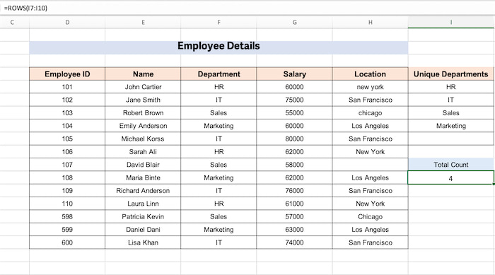
4. Go to an empty cell and use the ROWS Function. For Example, =ROWS(I7:I10). Excel will return a result = 4.

In case of counting the distinct values, you can also use the PIVOT Table apart from the Excels Filter option. We will discuss it in the next section.

Use Pivot Table To Count Distinct Values in Excel

Pivot table is a great integration for analyzing, and extracting insights from large datasets. Let’s assume you have a dataset with employee names and their respective departments. You want to find out how many distinct employees are there in each department.

Let’s look at an example dataset:

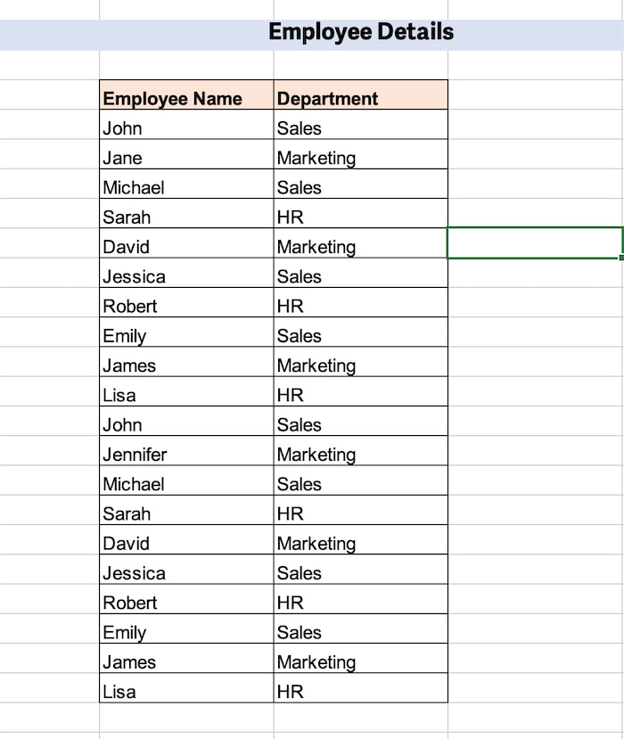
Here are the steps for creating a PivotTable to count distinct employees in each department:

1. Select Your Data

Click on any cell within your dataset. Then Go to the Insert tab in the Excel ribbon. Click on PivotTable.

2. Create PivotTable Dialog Box

In the Create PivotTable dialog box, ensure that the Table/Range field correctly identifies your dataset. Choose where you want the PivotTable to be placed (e.g., Existing Worksheet) and Click OK.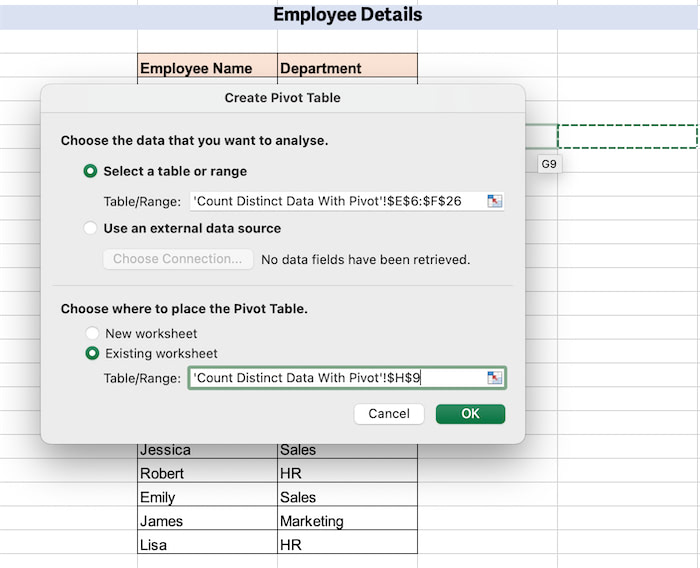

3. PivotTable Field List

You’ll see the PivotTable Field List on the right side of the screen. Drag and drop the Department field to the Rows section.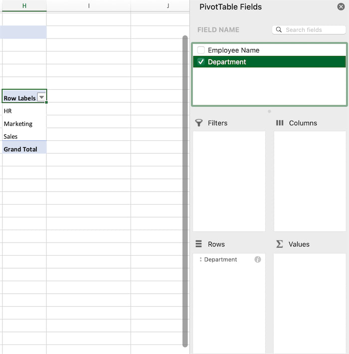

4. Count Distinct Employees

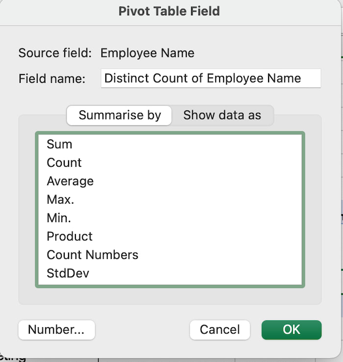
Drag and drop the Employee Name field to the Values section. By default, it will count the number of employees. To change this to count distinct values, follow these steps:

Click on the drop-down arrow next to Count of Employee Name in the Values section. Select Value Field Settings. In the Value Field Settings dialog box, select Distinct Count under the Summarize value field by dropdown menu. Click OK.

5. View Results

You should now see a PivotTable that shows the distinct count of employees in each department. In this example, you can see that there are 3 distinct employees in the HR department, 4 in Marketing, and 4 in Sales. If you want you can make Excel tables look good by changing the theme and color of the workbook.

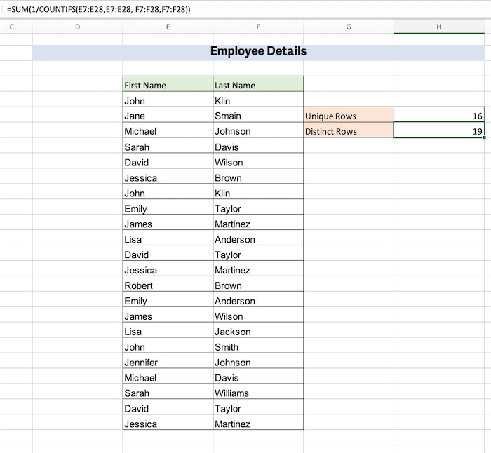
How To Count Unique And Distinct Rows Together in Excel

We will be still using the COUNTIFS Function to specify several columns to check for unique values. Here, we will set multiple criteria and based on those criteria, we will determine the unique and distinct values together.

In our dataset, we have the first and last name of our employees. We want to count the total number of Unique values and Distinct values here.

We will use the formulas:

For Unique Rows- =SUM(IF(COUNTIFS(E7:E16,E7:E16, F7:F16,F7:F16)=1,1,0))

For Distinct Rows- =SUM(1/COUNTIFS(E7:E28,E7:E28, F7:F28,F7:F28))

Note: In Excel 2007, there’s a limitation of 127 range/criteria pairs for COUNTIFS, whereas the limitations are significantly increased afterwards.

Limitations of COUNTIFS Function

There are approximately 8 limitations of the COUNTIF Function to count unique values. These limitations are listed below:

1. Criteria Must be in the Same Range: All the criteria in COUNTIFS must refer to the same range or an array of the same size. You can’t, for example, have one criterion in column A and another in column B.
2. AND Logic Only: COUNTIFS uses AND logic, meaning that all criteria must be met for a cell to be counted. There is no built-in way to use OR logic within a single COUNTIFS function. For OR logic, you’d need to use multiple COUNTIFS functions or alternative approaches.
3. Not Case-Sensitive: This point is a major limitation. By default, COUNTIFS is not case-sensitive. If you need a case-sensitive count, you’ll need to use additional functions like EXACT within an array formula.
4. Doesn’t Support Wildcards: Unlike some other Excel functions like COUNTIF, COUNTIFS doesn’t support wildcard characters like * or ? for partial matching.
5. Can’t Compare Arrays Directly: You can’t compare an array directly to a single value. For example, COUNTIFS(A1:A5, {1,2,3}) will not work. You would need to use multiple COUNTIFS functions or other methods.
6. Doesn’t Count Blank Cells Unless Specified: By default, COUNTIFS doesn’t count blank cells. If you want to include them, you need to explicitly add a criterion for blank cells.
7. Zero Capability to Count Distinct Values: For counting distinct values, you might need to use other functions or techniques. One common approach is to use helper columns with formulas like COUNTIF combined with array formulas or PivotTables for more complex scenarios.
8. Limited to 127 Pairs of Ranges and Criteria: In older versions of Excel (pre-Excel 2007), there’s a limitation of 127 range/criteria pairs for COUNTIFS. In modern versions of Excel, this limitation is significantly higher.

Note: If you have Excel 365 or Excel 2019, you can use the UNIQUE function along with COUNTA to count distinct values.

Conclusion

To sum it up, this guide gives you a solid grasp on how to count special types of values in Excel. We showed you how to find unique values (ones that appear just once) and distinct values (which include unique ones plus the first occurrence of duplicates).

You’ve learned practical methods using formulas like COUNTIFS, SUM, IF, ROWS, UNIQUE, ISNUMBER, and ISTEXT. These functions help you count different types of values in your data. Whether it’s text or numbers, you’re all set.

Remember, Excel doesn’t have a built-in way to count distinct values directly. But with the tricks shared here, you can breeze through it.

Lastly, be aware of some limits with the COUNTIFS function, and explore workarounds when things get complex. Armed with these techniques, you’re well-prepared to handle unique and distinct value calculations like a pro!