
Microsoft Excel gives a variety of choices and ways to make our job simpler. In this post, we are going to demonstrate many ways of using Excel through which you can do the equation of if one cell equals another then return another cell very easily.
Suppose you have three values in three different columns. Now, you want to get the value of column three in a different cell only if column one and column two values are the same! So, how can you do that?
You can easily do that by using many functions like If, LOOKUP, IndexMatch function combo, and so on. So, continue reading this post until the end to learn in detail.
5 Easy Ways to Get If One Cell Equals Another Then Return Another Cell
By following the below methods, you can get a cell value if one cell equals another then return another cell in Excel:
1. By Using the IF Function
If you want to get a cell value if one cell equals another then return another cell in Excel, then using the IF function would be the very simple and easy way to do that. As we already know, IF is one of the most basic functions in Excel, and it is mainly used to make a logical comparison between the two numbers.
Using the IF function, we will be able to compare one cell value with the other and get the value of a particular cell in this manner.
But, before moving on to the main procedures, it would be great if you learned more about this formula. Here’s how the function’s syntax is written out:
=IF (logical_Condition, [value_if_true], [value_if_false])
As you can see in the formula, in the logical_Condition section, we will have to enter the condition that we will be using to compare the values. And in the [value_if_true] and [value_if_false] sections of the formula, we are going to describe what will happen if the values following the comparison are True or False, respectively.
Now, follow the below steps carefully to know how you can use the formula in Excel:
- Open the Excel spreadsheet and select your desired cell where you want to get the output.
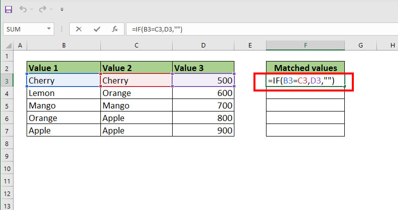
- In our case, we chose the F3 cell, as you can see in the screenshot below. Now, type the following formula carefully. =IF(B3=C3,D3,””)
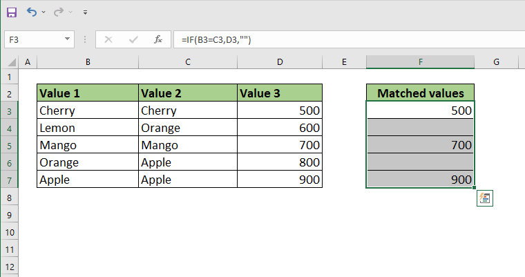
- Once you are done, hit the Enter button on your keyboard, and you should see the value 500 appear on the F4 cell.
- Now copy and paste the formula in the below remaining cells by dragging the Fill Handle (Plus icon located in the bottom right corner) option.
Detailed Explanation of the Formula
To begin, we are going to compare the Fruits Names in every field of the Value 1 and Value 2 columns using the condition B3=C3. If the condition is met, the numbers from the Value 3 column will be placed into the Matched Values column. Otherwise, the condition is false, and nothing will be written on that cell.
Part 2: Now we have copied and pasted the formula all the way down to the F7 cell by dragging the Fill Handle (Plus icon located in the bottom right corner) option, and we will see the numbers 500, 700, and 900 written on the cells according to the formula.
2. By Using the IF Function and Formula
And here is an example of another case. Consider the following scenario: you have two columns, and you will need to get the cell value depending on the other cell if it includes a specified text string, such as the word X.
Using the same IF statement as before, we can utilize the same formula and display the results in a different cell depending on the case we are dealing with. Consider the same dataset that was utilized in the previous step, except that this time we are going to change the Price if the Flag value is not X.
And guess what? Our new price will be three times bigger as much as the existing price, which you are going to see below.
So, to do that, follow the below steps carefully:
- Open the Excel spreadsheet and select your desired cell where you want to get the output.
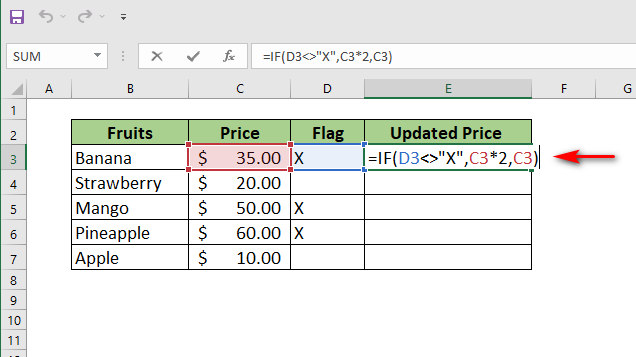
- In our case, we chose the E3 cell in the Updated Price column, as you can see in the screenshot below. Now, type the following formula carefully. =IF(D3<>”X”,C3*2,C3)
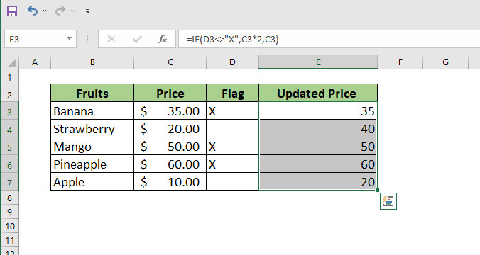
- Once you are done, hit the Enter button on your keyboard, and you should see the value 35 appear on the E3 cell.
- Now copy and paste the formula in the below remaining cells by dragging the Fill Handle (Plus icon located in the bottom right corner) option.
Pro Tip: Did you know, in the column Flag, you can actually put the word X automatically by using a formula? Suppose you want to put the word X if the value of the price is greater than 20 and you don’t want to increase anymore. So, in that case, you can write the formula =IF(C3>20,”X”,””) in cell D3 and drag it down to the remaining cells by using the Fill Handle option.
Detailed Explanation of the Formula
When we are using the D4<>” X” function in the formula =IF(D3<>”X”,C3*2,C3), we are analyzing if the value of Flag is not equal to X or not. If the requirement is met, the price will be tripled; otherwise, the price will stay unchanged.
And in this way, you can get a cell value If one cell equals another then return another cell by using the IF function and formula.
3. By Using the LOOKUP Function
When it comes to looking for anything in Excel, the LOOKUP method will be the most appropriate option to apply. When we use this function, we may look for anything vertically or horizontally inside criteria within a specified range. And VLOOKUP and HLOOKUP formulas in Excel are designed specifically for these kinds of situations.
VLOOKUP Function:
Now just like the IF function, let’s take a look at the most basic form of the VLOOKUP function. The function’s syntax is as follows:
=VLOOKUP (lookup_value, table_array, col_index_num, [range_lookup])
In the section lookup_value, we will enter the value which we will be looking for in the first column of a table.
In the section table_array, we will enter the range of the table.
The section col_index_num is the table’s column index number of the table that we will use to get a value.
The section range_lookup is the last part that is used to indicate the optional range.
Now, in our demo spreadsheet, we are going to pull the price of fruit in cell G3.
So, to do that, follow the below steps carefully:
- Open the Excel spreadsheet and select your desired cell where you want to get the output.
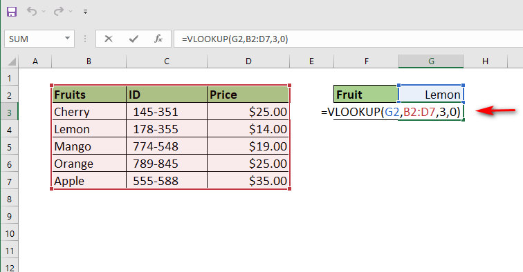
- In our case, we chose the G3 cell in the Price row, as you can see in the screenshot below. Now, type the following formula carefully. =VLOOKUP(G2,B2:D7,3,0)
- Once you are done, hit the Enter button on your keyboard, and you should see the value 14 appear on the G3 cell.
- Now copy and paste the formula in the below remaining cells by dragging the Fill Handle (Plus icon located in the bottom right corner) option.
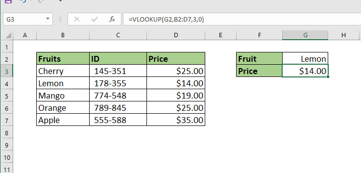
After we have carefully done all the steps above, when we type any name of the fruits from column B, the price will automatically be entered in the G3 cell. Isn’t that amazing?
Detailed Explanation of the Formula
In the formula =VLOOKUP(G2,B2:D7,3,0) we have first entered G2 as the value. Because we want to get data according to the value of this cell. Then we selected the whole table from B2 to D7 in the table_array section. As we want to get data from that table. Next, now that we want to get the price of the fruits, we will enter 3 in the col_index_num section. Because the price column is in number 3. Then we have entered 0 because we want to get the exact value.
After that, the price of the fruit will be entered automatically in the Price field.
HLOOKUP Function:
Now that we have understood the VLOOKUP function, it’s time to take a look at the HLOOKUP function. Because VLOOKUP is only built for vertically aligned syntax.
So, what if your spreadsheet is designed horizontally? In that case, you can use the HLOOKUP function to do the job.
Now then, let’s see the HLOOKUP functions syntax:
=HLOOKUP (lookup_value, table_array, row_index_num, [range_lookup])
The syntax is pretty similar to the VLOOKUP function, except, instead of col_index_num, there is row_index_num. So, I don’t think we should break down the formula.
Now, just like the previous steps of the VLOOKUP function, open the spreadsheet and select the cell where you want to get the value.
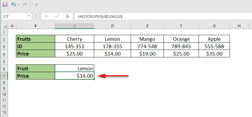
Then enter the following formula carefully: =HLOOKUP(C6,B2:G4,3,0)
The price of that specific fruit should appear right after you press the Enter button on your keyboard.
4. By Using The INDEX and MATCH Functions
This method is just like the previous method, but the only difference between this part and the last one is that we will not be using the LOOKUP function. Instead, we will be using the INDEX function.
Because the INDEX and MATCH functions will perform the same job as the LOOKUP function, in addition, the information will be the same as it is now. So, you won’t have to edit a single thing.
Now, before we go to the demonstration, let us just take a closer look at the contents of these two functions.
=INDEX (array, row_number, [col_number], [area_number])
The highest number of parameters that this function may handle is four, while the lowest number of parameters is two. In the first portion of its field, it asks for the range of cells from which we will extract the value of the index.
Afterward, there’s the row number of the referencing or matching value. The last two inputs are optional, and they allow us to create or declare the column position from which the matching data will be obtained, as well as the area range number.
=MATCH (lookup_value, lookup_array, [match_type])
The MATCH function is yet another frequently utilized function. In the first parameter, we enter the value that we are searching for or matching. Our required data will be located in the second array, which is referred to as a lookup_array. The match_type is the last consideration. We can manipulate matching based on various match type values.
Some of the match_type values are given below:
1 = The value of 1 indicates that the lookup function should seek for the biggest value less than or equal to the lookup parameter value.
0 = Using a match type of 0 will return the result that is identical to the lookup value, which is what we want.
-1 = The lowest value larger than or equal to the lookup value will be matched by this.
Now that we understand the syntax of the formula, it’s time to put all these into action.
So, to do that, follow the below steps carefully:
- Open the Excel spreadsheet and select your desired cell where you want to get the output.
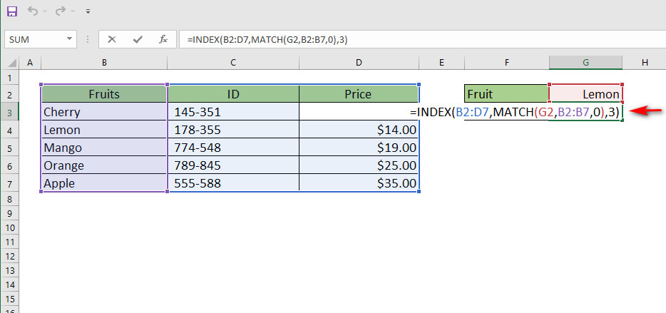
- In our case, we chose the G3 cell in the Price row as you can see in the screenshot below. Now, type the following formula carefully. =INDEX(B2:D7,MATCH(G2,B2:B7,0),3)
- Once you are done, hit the Enter button on your keyboard and you should see the value 14 appear on the G3 cell.
- Now copy and paste the formula in the below remaining cells by dragging the Fill Handle (Plus icon located in the bottom right corner) option.

Detailed Explanation of the Formula
In the section, MATCH(G2,B2:B7,0) we will attempt to match the value that is now in the G2 cell with the value that is currently in the B2 to B7 range in our lookup table. And since we took into consideration the precise match, the value 0 is given to the last parameter.
And now, in the full formula, =INDEX(B2:D7,MATCH(G2,B2:B7,0),3), I’ve given a range of cells to the first section of the equation. Then the MATCH function will be used to compute the value that matches the criteria. Finally, the number 3 is utilized because we wish to get information from the third column in our lookup table.
In this way, the IndexMatch function works.
5. Pull Values From Another Sheet if the is a Match
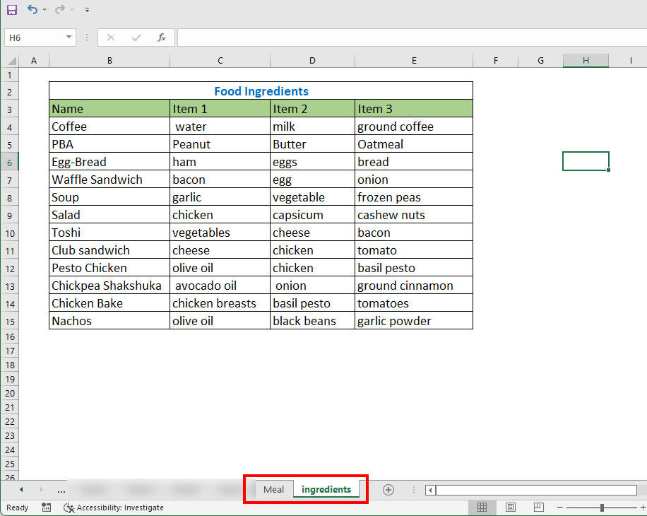
Now in this method, we are going to show you how you can pull values from another sheet if one cell is equal to another. In this example, we will use a dummy weekly meal planning table and another sheet where we put all the ingredients. Our plan is to pull the ingredients in the first sheet.
So, follow the below steps carefully to do that:
- We opened the Meal worksheet and entered the following formula in the C13 cell: =VLOOKUP($B13,ingredients!$B4:$E15,2,FALSE)
- Then we copied and pasted the remaining three cells. But instead of 2 in col-index-num, we entered 3 in D13 and 4 in E13 cell.
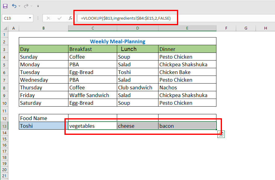
Now, according to the B13 cell, the ingredients from the other sheet will be entered in the following cells.
Hence, as the formula is VLOOKUP, and we already explained this formula, we don’t think we should repeat the explanation twice.
Conclusion
So, these were the formulas to compare one cell with another and return another cell in Excel. We tried to show all the techniques with their relevant samples. In addition, I have covered the basics of this function as well as the most often encountered format codes for these formulas as well. We hope this article has helped you to learn how you can do the equation of if one cell equals another then return another cell in Excel.

