How To SUM Only Filtered Data in Excel [Advanced Functions]

1+2=3. It’s a simple addition that can be done using the SUM function in Excel.

However, Excel has more to offer.

There are some advanced SUM functions that can ease more complex tasks.

In this post, we will show you how to SUM visible rows in a filtered list in Excel. So, tag along.

Filtering Data in Excel

Excel’s Filter function allows you to narrow down a large data set to only show specific information that you’re interested in.

Let’s get nostalgic for a bit. You had been into science labs filtering solutions with a filter paper. The filter paper grab holds some of the particles and the rest of the solution is placed in a beaker.

Similarly, Excel’s filtering data easily focuses on a particular subset of your data set and excludes the rest.

To illustrate how filtering works in Excel, let’s work with a sample data set.

Imagine you have a spreadsheet that contains data on employee performance, including their name, department, date of hire, and performance score. Here’s what the data might look like:

Name	Department	Hiring Date	Performance Score
Sadmin Khan	Pharmacy	15-04-2023	80
Polash Chakraborty	HR	16-04-2023	90
Daniel Wang	Sales	17-04-2023	75
Tripathy Saha	Marketing	18-04-2023	65

There are two ways to filter this dataset.

Using the Filter function.
Inserting a table. The table will create alternate shades, and you can make Excel tables look good the way you want.

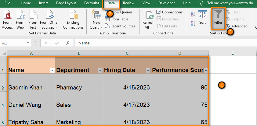
Let’s look at the first way. To use the Filter function, select the whole dataset, then go to the Data Tab and select the Filter option. This will create a dropdown menu in all the headers.

Alternatively, select the whole dataset and click on the Insert Tab. Select the Table option and check mark the “My Table has headers” option.

How to use SUM Function in Excel

The syntax of the SUM Function is-

=SUM(number 1, [number 2], …)

You can either select specific cells or a range of cells for addition using this function. For Example, =SUM(A1,A2,A3), or =SUM(A1:A10), or =SUM(A1, A4:A11).

Create a dataset and type the formula using the equals to sign (=). Press Enter for Excel to return a result.

Problem With The SUM Function

The only problem with the SUM function is that this function adds all the hidden and unhidden values. So, if you have a hidden row, Excel will calculate that row too.

Let’s look at an example.

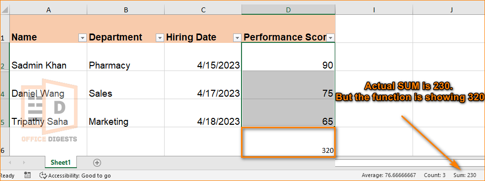
The total of D2, D4, D5 cells is 220. But, the SUM function shows the result 310. This is because the D3 cell was hidden and the SUM Function calculated that number too.

Excel’s SUM function couldn’t count the result of filtered data.

Note: If the filtered data is gathered first and then you apply the SUM function, only then Excel will return the accurate result. Condition applied, you have to select the cells manually.

Now, you know that you cannot add the filtered data simply.

Don’t worry. We will now show you the exact way to do so.

How to Sum Only Filtered or Visible Cells in Excel

There are two such functions which are able to filter only visible cells. The two related functions are:

AGGREGATE Function
SUBTOTAL Function

Here are the ways to sum only filtered or visible cells:

1. Use the AGGREGATE Function

An aggregate function in Excel is a function that performs a calculation on a group of values and returns a single result.

The main aim of using this function is to summarize the data in an advanced way. There are approximately nineteen function values and seven options inside this AGGREGATE syntax. The array present in this function is not the same as creating a table array argument.

Interesting fact is that this function doesn’t add the hidden rows or columns.

The syntax for AGGREGATE Function is:

=AGGREGATE(function_number, options, array…)

Some examples of aggregate functions in Excel include SUM, AVERAGE, MAX, MIN, COUNT, COUNTA, COUNTIF…

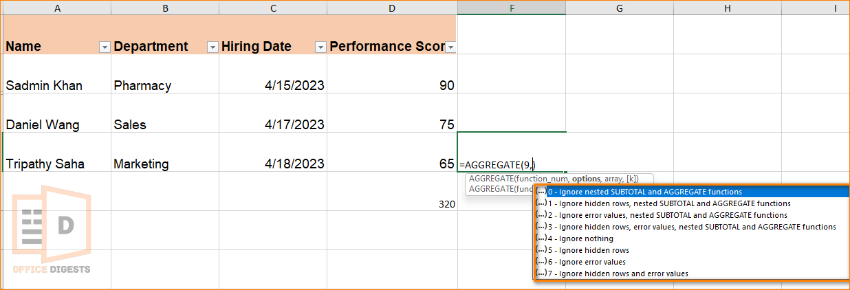
Here are the steps of using the AGGREGATE function in Excel:

Select a blank cell where you want to display the sum.
Type =AGGREGATE(9, 5, range) in the formula bar where range is the cells you want to sum.
Press Enter to calculate the sum.

Apart from using the AGGREGATE function, there’s another function known as the SUBTOTAL function.

2. Apply the SUBTOTAL Function

SUBTOTAL works similarly to the AGGREGATE functions. The difference is that SUBTOTAL function allows 22 options. Function numbers are listed once you type =SUBTOTAL( in the active cell.

The syntax for SUBTOTAL function is:

=SUBTOTAL(function_number, range)

where range indicates the cells you want to sum, or average, or even count.

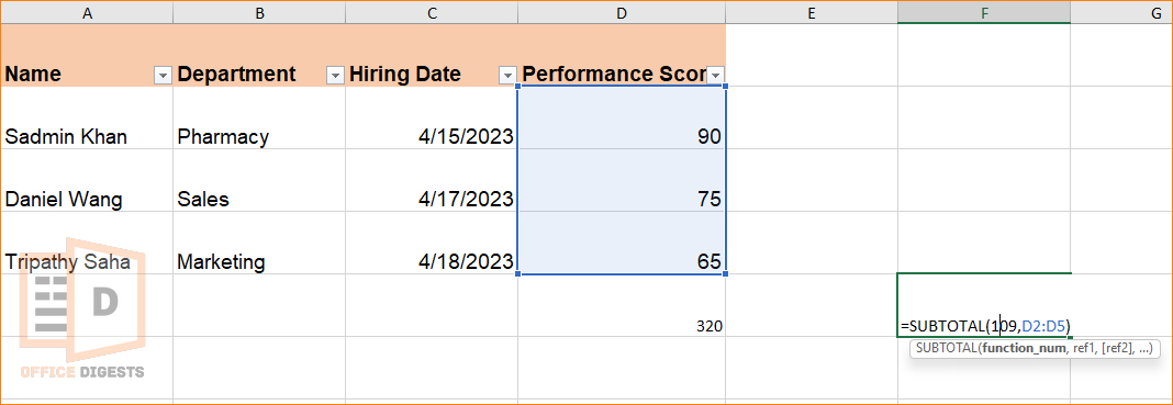
Here are the steps of using the SUBTOTAL function in Excel:

Select a blank cell where you want to insert the formula.
Type =SUBTOTAL(109, range), where range indicates the cells you want to sum up.

Notice one thing.

There were two sum function numbers (9 and 109). The difference between those two numbers is that the number 9 SUM adds the values of both hidden and unhidden cells.

Whereas, the number 109 SUM adds only the visible cell values – which is what we want!

Whether you choose the number 9 option or the 109 option depends on the criteria.

So, use the SUBTOTAL on Filtered data based on criteria!

The next method is a bonus one. We will show you how to sum visible columns in excel using VBA.

How To Sum Only Filtered (Visible) Cells in Excel With VBA

Previously you have dealt with advanced sum functions in Excel. Now, we will be using a user-defined VBA Function.

Preliminary requirements:

Enable VBA in Excel
Ensure the workbook is macros-enabled.

Here are the steps to sum only filtered data in Excel using VBA:

Go to the Developer Tab and select the Visual Basic Option.
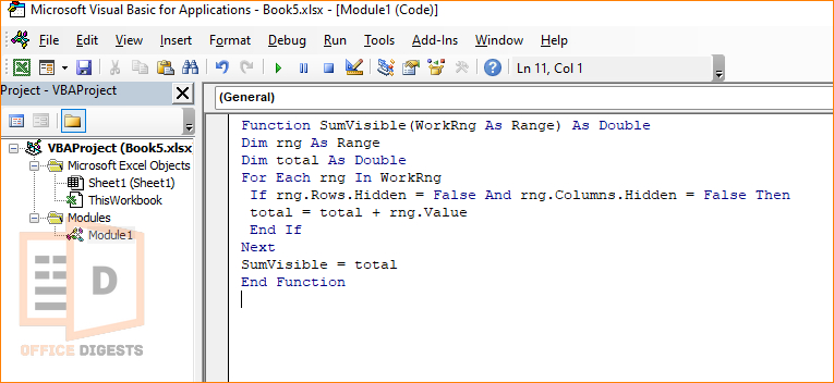
Insert a new module and paste the following code-

Function SumVisible(WorkRng As Range) As Double
Dim rng As Range
Dim total As Double
For Each rng In WorkRng
 If rng.Rows.Hidden = False And rng.Columns.Hidden = False Then
 total = total + rng.Value
 End If
Next
SumVisible = total
End Function

Run the Function using F5 or pressing the Run button.

Explanation of the Code:

The function first declares two variables: a Range object named “rng” and a Double data type named “total”. The “rng” variable will be used to loop through each cell in the input range, and the “total” variable will keep track of the sum of the visible cells.

In short,

If the cell is visible, its value is added to the “total” variable.

After looping through all the cells in the input range, the function returns the value of “total” as the sum of the visible filtered cells.

How to Use the SumVisible Function in Excel?

After pasting the code in the module, run the code using F5. Then return to the Excel worksheet. Select any cell where you want to insert the formula and type =SumVisible(range of cells), where range of cells includes the cells which we want for addition.

For Example:

=SumVisible(A5:A12)

Then press Enter.

Here, all the visible cells will be added. If you want to add any unhidden columns then you have to unhide columns in Excel and then use the SumVisible formula.

But sometimes, you may notice that the SUM function returns a result of 0.

Excel SUM Function Returns 0?

The SUM Function only returns a value of 0 if there is any presence of circular references. To fix the circular reference, either shift the formula to a different location. Or, change the range of cells. You can even enable iterative calculation to fix the error.

FAQ

Q: How to sum selected cells in Excel?
A: Select any cell and type =SUM. Now select the cells you want to add and separate them with commas. For Example: =SUM(A2, A4, A5). Press Enter to execute the formula.

Conclusion

Excel has a huge collection of functions. Just like the SUM Function. Normally, we use this formula to add all the values in a column.

But, in most cases, we filter our dataset. If we want to sum up all the filtered data, then we need advanced sum functions just like the SUBTOTAL and AGGREGATE.