
The keyboard shortcuts to highlight rows and columns in Excel are Shift+Spacebar and Control+Space Bar respectively in both Mac and Windows.
And to highlight the entire active worksheet, you have to press Control+A button altogether.
But, that’s not always the easy case.
If you have a small dataset, you can easily hover your eyes spotlighting the necessary value. However, for a large dataset, it’s a different scenario.
What if we tell you there are ways to highlight active rows in Excel based on cell value. To know more, read the whole post.

Why is Highlighting Rows & Columns Important?
To find something in seconds, of course…
However, As W. H. Auden said, “There’s more than meets the eye”.
So, here are some of the reasons why you should often embrace highlighting active cells:
Data Analysis
By highlighting specific rows and columns, you can quickly identify trends and patterns in your data. For example, Consider highlighting students’ grades as green if their marks are greater than or equal to 80.

Quick Navigation
When working with a large spreadsheet, marking rows and columns can help you navigate and find the information you need quickly.
It allows you to easily jump to different parts of the spreadsheet without having to scroll through the entire document!
Perform Immediate Action
There are times when you have to make a quick decision. Deleting, copying, and moving highlighted cells will become helpful in that case.
You can select multiple rows and perform necessary actions when needed.
Automatically Highlight and Refresh Active Rows in Excel
Using conditional formatting and macros are two ways of highlighting a cell. However, when you change cells, the highlighted portion doesn’t change. It’s common if you are a beginner in Excel.
If you want to reach the intermediate level, tag along.
Here are the steps to automatically highlight and refresh rows in Excel:
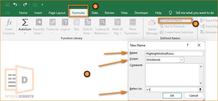
1. Define a Name For Your Worksheet
Organize all your data in a single spreadsheet. After that, fix the headers (if any).
Now go to the Formulas Tab from the ribbon bar and click on Define Name. Type a name in the Name Dialog Box. Let’s say HighlightActiveRows. Type =1 in the Refers to box and select the scope Workbook. Press OK. This process will now define a name to your active worksheet.
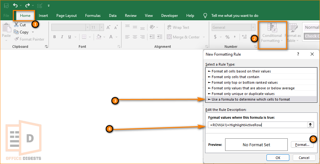
2. Apply Conditional Formatting
Conditional formatting makes particular cells easier to identify. To apply this feature, go to the Home Tab and Select Conditional Formatting and click on New rule.
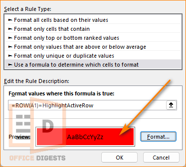
Use a formula to determine which cells to format and type =ROW(A1)=HighlightActiveRow where the Format values where this formula is true box is present.
Click on the format button and select the background color. Click OK to preview the full formatting. Select OK again.
3. Apply the VBA Code For Automatic Refreshing
Press Alt+F11 to open the Visual Basic box. If the Developer Option is not present, then you should first enable the VBA option in Excel. After that, insert a new module and paste the following code-
Private Sub Worksheet_SelectionChange(ByVal Target As Range)
With ThisWorkbook.Names("HighlightActiveRow")
.Name = "HighlightActiveRow"
.RefersToR1C1 = "=" & ActiveCell.Row
End With
End Sub
Now Run the code using F5 and return to your spreadsheet.
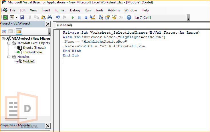
Note: Notice that the Define name must match with the code Workbook name in code line 2 and 3.
4. Test The Code
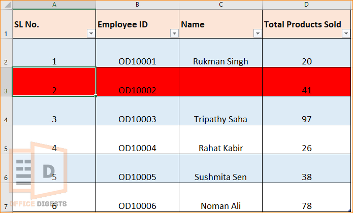
Try selecting any cell. This will automatically highlight the whole row. You don’t need to press the F9 button to refresh the worksheet. With this VBA code, you can easily highlight the entire row in Excel when a cell is selected.
Highlight Rows Based on a Text Criteria For Mac Users
For Mac users, Conditional formatting interface is not the same as Windows OS. Select the whole dataset using Ctrl+A or Command+A button and then go to the Home Tab to select the Conditional Formatting Option.
Click on the New Rule option and Select the Classic Style. By default the classic style is set to “Only format top or bottom ranked values”. Change the option to Use a formula to determine which cells to format. Now, type =$A2=”Ron” in the blank box.
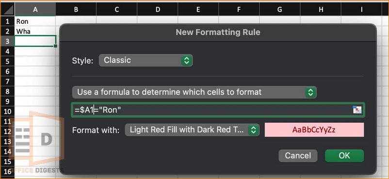
This formula indicates that we want to highlight the entire row if any cell contains the text Ron. Format the cells with any of your preferred background colors and Press OK.
Result: All rows containing the text value “Ron” will be highlighted in red.
How To Alternate Highlight Rows in Excel
To create alternate shades in cells, you have to insert a table. It’s really easy if you already have a dataset in your worksheet.
We have made a complete tutorial on making Excel tables look so good that you can ace your job presentation!
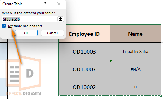
Now, to highlight alternate rows, select the dataset and go to Insert > Table. If your table has headers, then select the “My Table has headers” option. Click OK. Now you have alternate coloring rows.
And now, you can SUM cells based on the background colors.
Highlight Columns in Excel
To highlight an entire column in Excel, press the shortcut key Control+Spacebar for both Mac and Windows users.
Normally marking rows is common because all the necessary data are present row-wise for a particular criterion.
However, in some cases you may want to highlight the entire column. Either press on the whole column itself if your mouse cursor is just beneath the Ribbon Bar. And if you are in the middle of your dataset, just press Ctrl+Space.
Ctrl+Space Not Working to Highlight Columns on Excel For Mac?
You are unable to use the keyboard shortcut key in excel for mac because by default your MacBook is using that same shortcut key for other purposes.
So, what to do to fix such problems?
Well, go to the System Settings on your Mac and scroll down. Click on the Keyboard option. Select keyboard shortcuts under Keyboard Navigation. Go to Input Sources and uncheck the option that says “Select the Previous Input Source”. 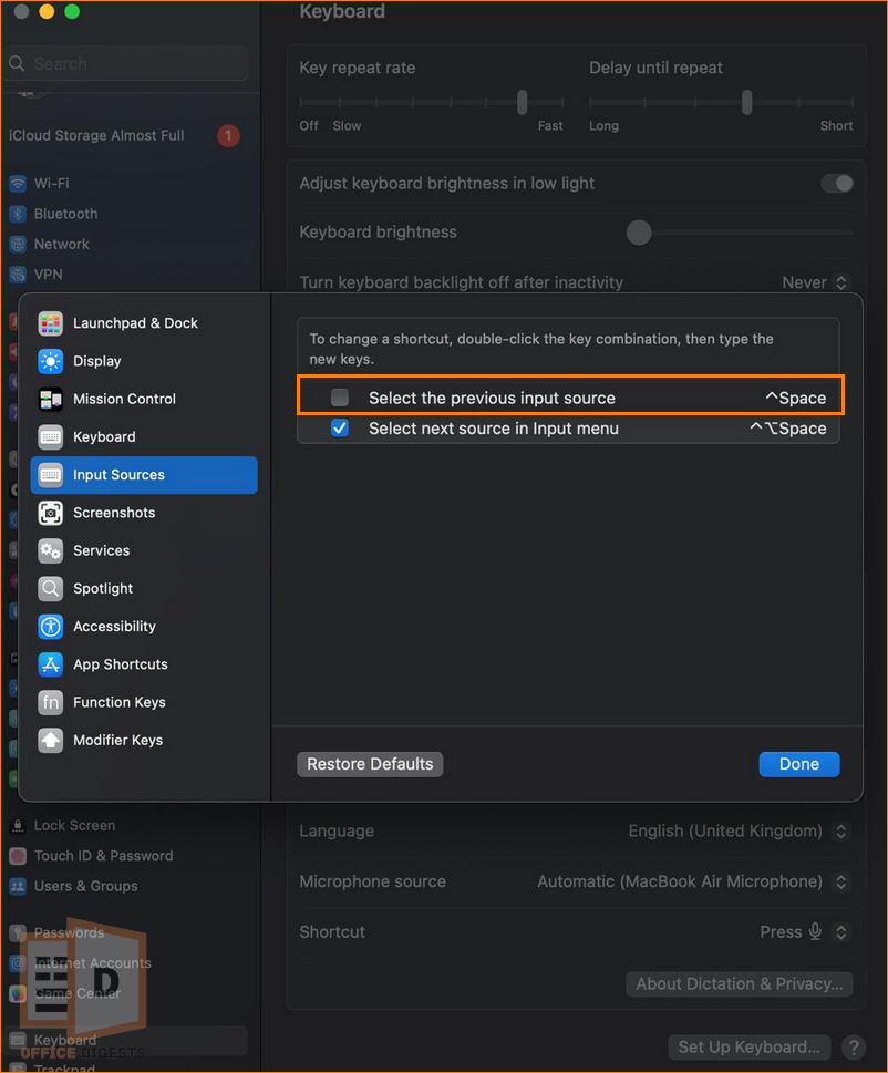
Notice that your Mac is using the same command ^Space as Excel’s column highlighting command. Click on Done to fix the issue.
FAQ
Q: Can Excel auto highlight rows?
A: Excel doesn’t auto highlight rows. You have to use Excel’s built-in feature “Conditional Formatting” or use a macro to highlight the selected rows automatically. Do ensure saving the file as a macro-enabled file.
Q: How to color rows in Excel?
A: To color rows, you have to use Conditional formatting. Go to the Home tab and select the conditional formatting option. Select the option that says Highlight cell rules. If you want to highlight cells that contain text “Leon” then click on the option “Text that Contains…”. All cells containing the text “Leon” will be highlighted.
Q: How to highlight an entire row in Excel with Conditional Formatting?
A: Use a formula to determine which cells to format in the Conditional Formatting New Rule Format box to mark an entire row.
Conclusion
We have provided the easiest and the most convenient way of highlighting rows in Excel.
You can utilize these steps and can mark rows in different colors based on multiple conditions. Not only that, you can even highlight blank cells using this simple technique!

