How To Create Dynamic Map Chart in Excel [+Free Templates]

So, are you still using those boring bar and pie charts in Excel for your presentation? If you have ever felt that your Excel sheets needed a dash of excitement, you’re in the right place.

We are about to dive headfirst into the realm of Dynamic Map Charts. Tag along as your numbers come to life, dancing and prancing across the world map.

It’s not just a chart, it’s a visual fiesta!

So buckle up because, in this tutorial, we are going to show you how to create a dynamic map in Excel that will take your data presentation to a whole new level.

What is an Excel Map Chart?

A Map chart in Excel is a visual tool for comparing values and categories across different geographical regions. You can get the best representation when dealing with data associated with geographic entities like countries, states, or postal codes.

Map charts show distinct color schemes. For Example: the numerical values are of the same color with different shades (the higher the value the darker the color). Whereas, the categories are colored differently.

You might ask:

When to use Map charts?

Well, honestly speaking, this map feature is particularly valuable for tasks like regional sales analysis, demographic studies, or any scenario where location-based data is significant.

PRO TIP: Maps work best with geographical data (regions, provinces, states, and revenues) in separate columns.

Now, let’s look at the process of creating a map chart. But Before that,

Get Hands-On: Download the Practice Workbook and Work Along with the Steps

You can click below to download the practice workbook (From Google Sheets to Excel) and follow along with the step-by-step instructions.

Download Map Chart in Excel.xlsx

How to Create a Dynamic Map in Excel

In this section, we will teach you how to use the Key Performance Indicator (KPI) by geography for our company’s product and create an interactive map accordingly.

In short:

We are adding interactivity to the map.

So, let’s look at our dataset.

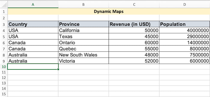
We want to visualize our dataset on a map. Also, we want to ensure that the map is dynamic (that is, data will change upon changing the country). The data includes information about different countries, their provinces, the revenue generated in each province/state (in USD), and the population of each state.

Note: We will use the Scatter Plot with a background image to create a map chart. And then switch the Scatter plot to a Bubble Chart.

Bubble charts are basically the same as Scatter plots with some additional dimensions.

So, here are the steps to create a dynamic map chart in Excel:

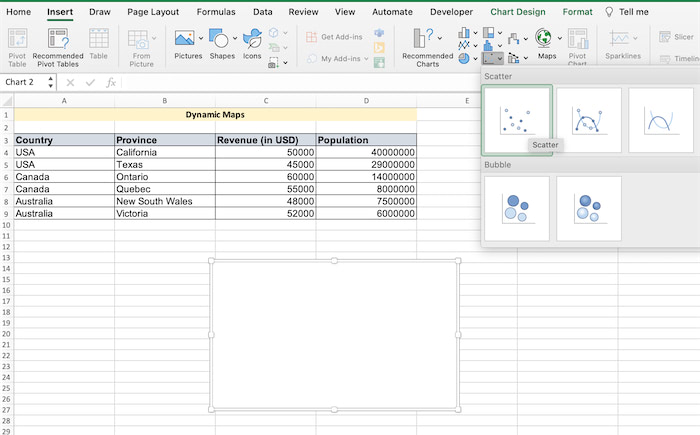
1. Insert a Blank Scatter Plot

Click outside your dataset on any cell and go to the Insert Tab from the ribbon bar. Click on the drop-down menu of the plots (beside the Recommended Charts Section). Select the Scatterplot option.

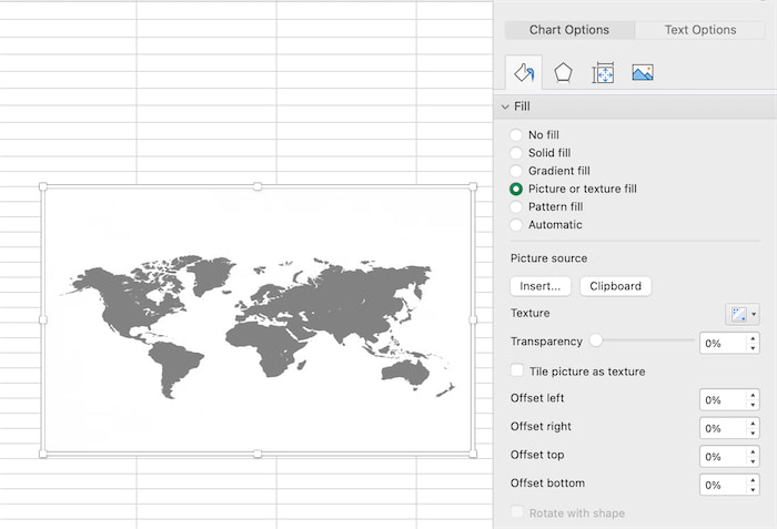
Double-click on the blank chart and fill the chart with a background image. Here we will be using an image from online. We used a free vector world map in gray color.

For easy formatting, remove gridlines from your Excel workbook. Go to the View Tab and unmark the grid lines option.

Now, tweak some minor settings.

Set the Transparency of the image to nearly 70%
Lock aspect ratio of the chart
Remove the outlines from the map

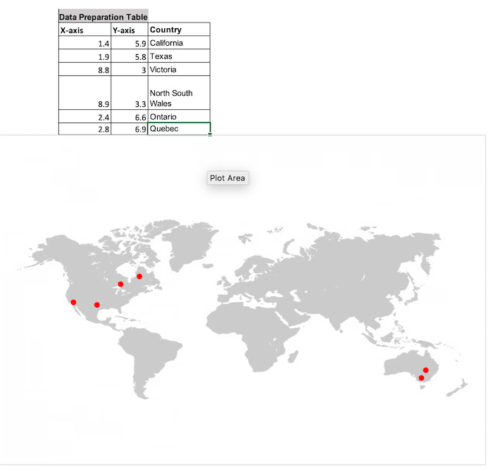
2. Plot the Points into the Map

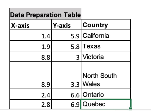
To plot the points inside a filled image of a map, we have to prepare our dataset. Mostly, we have to fix our X and Y-axis to a certain value set. Let’s say the values are from 0 to 10 for both the axes.

Note: We have to prepare a data table that’s going to sit on the map. Don’t change the raw data table.

In short:
The raw data table is going to feed the Data Preparation Table (DPT) and the DPT is going to feed the map.

So, let’s prepare our DPT. In our case, we are showing the XY Axis based on the province, and not the country. We will add a third-dimension for accurate data.

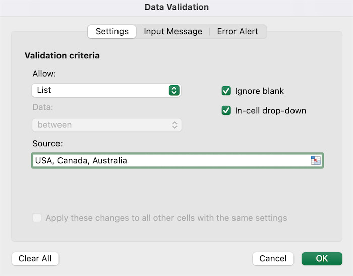
For the third-dimension, we will create a data validation list for selecting the country region. To do so, select a blank cell and go to the Data Tab. Select the Data Validation option and set the validation criteria to LIst. Inside the Source Tab, write the three country’s name (USA, Australia, Canada).

Now, to see the revenues based on the country and provinces, we will use the SUMIFS Formula. Notice that we are not adding anything, just setting up the criteria.

So, our formula will be-

=SUMIFS($C$4:$C$9,$B$4:$B$9,G5,$A$4:$A$9,$J$4)

Notice that we locked the cells to avoid errors. If you are a beginner and don’t know what the dollar sign means in Excel, then we suggest you learn the Cell Referencing first.

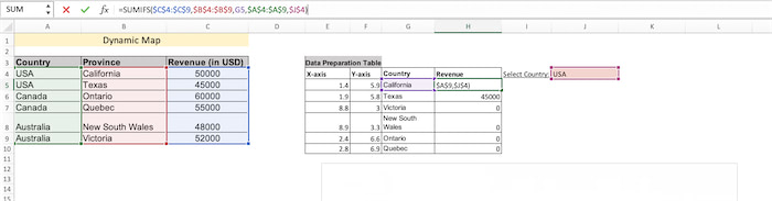
We selected two criteria. One is the country, and the other is the province. Now, since we added another dimension (revenue), we will now convert the scatter plot into a different chart.

3. Convert the Scatter Plot into a Bubble Chart

A bubble chart in Excel is a type of chart that displays three sets of data on a two-dimensional graph. The added element alongside the X and Y axis is the Bubble size.

Right-click on the graph and change the chart type to XY (Scatter) > Bubble. You can either choose the 2D variation or the 3D one according to your convenience.

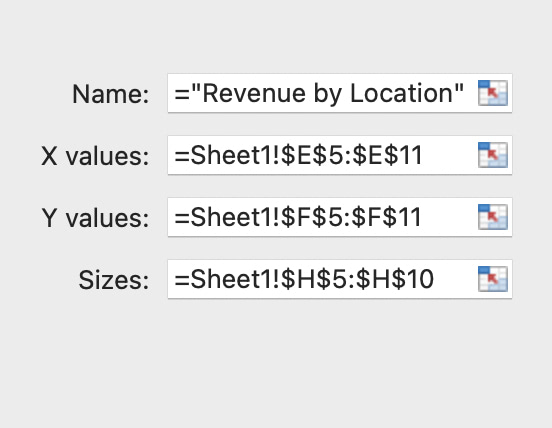
At first, there will be big chunks of bubbles because initially Excel won’t understand the positions of each element. To make Excel understand the problem, we have to right-click on the chart, select Data and put the Revenue series inside the Bubble Sizes range.

Whenever you change the country from the drop-down list, the graph changes dynamically. This type of chart is called an interactive map chart.

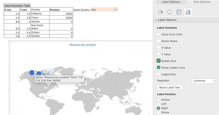
Click on the bubbles and customize the width of them to around 40 for a better look. Also, make the following necessary changes:

Add Data labels based on Bubble Size (Revenue)
Change the Number Format and Link it to Source (optional).

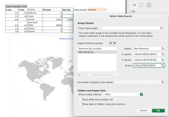
Now, since the data is very close to each other, we want to find out the max revenue of them only. For that, we will use the IF function.

So, let’s create another column and add the following formula:

=IF(H5=MAX($H$5:$H$10),H5,””)

Press Enter and Drag the column to apply the formula to other cells. Now, whenever you change the location, the max revenue will show the largest number.

Let’s add this situation into the graph. Right-click on the graph and select add data. Click on the (+) icon and add the X,Y, and size range. This time set the size range for the Max Revenue. Click OK when you are done.

So, this is how you create a map in Excel using the Scatter Plot Method.

Note: There is an in-built Map Option in Excel if you have Office 2019 or Microsoft 365 subscription.

Let’s look at the alternative and easy way.

Create Bing Map Chart in Excel (For Microsoft 365 Users)

You are lucky if you have Microsoft Excel 2019 or MS Office 365 subscription. In these two versions, you don’t need to create a map with such hassle. With just a click of a button you can create this chart easily.

Here are the steps to create a bing map in Excel:

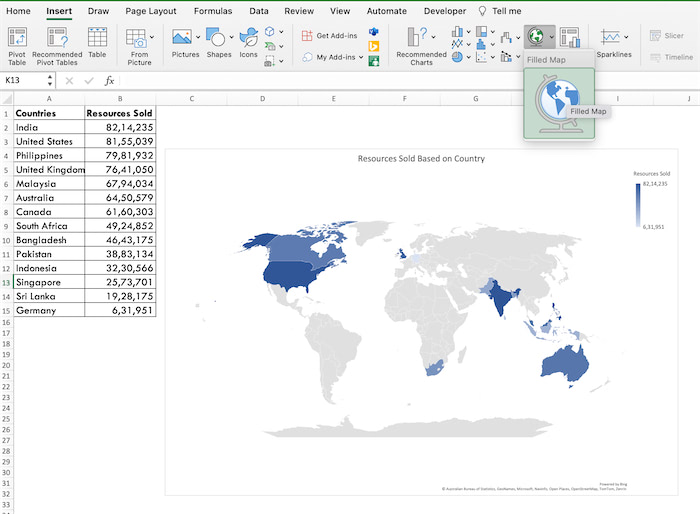
Select the dataset and go to the Insert Tab.
Find the Global Map icon and select it.
Accept the pop-up message ‘Data needed for your map will be sent to Bing’.
Click OK and your map is ready.

Result: The map will look something like this:

Final Words

In this guide, we taught two alternative ways to create a map in Excel. One is for Office 365 users and the other is for those who use Excel 2016 or lower.

For the 365 users, you will get the map option by default. Whereas, for other Excel users, you need to create a scatterplot and convert it into a bubble chart later onwards.