
Visual cues make all the difference. In an Excel data full of black texts, it’s hard to draw attention.
Suppose you have a large annual financial dataset for your company. Amidst the columns of revenues, expenses, and projections, lies some undetected problems. But what if you could elevate this data-driven journey further?
An integral part of effective data communication is presentation. So, highlighting cells in red creates an impactful way to draw attention and enhance data interpretation.
In this post, we will guide you the exact ways to make negative numbers red in Excel so that you can plan your next budget without errors.

Highlight Negative Numbers in Red Using Number Formatting
Whether you are converting negative numbers to positive in Excel, or highlighting those negative numbers, you need to use the Number formatting.
Number formatting is like a disguise that you apply to the cell. The actual number behind the cell is shown in the formula bar.
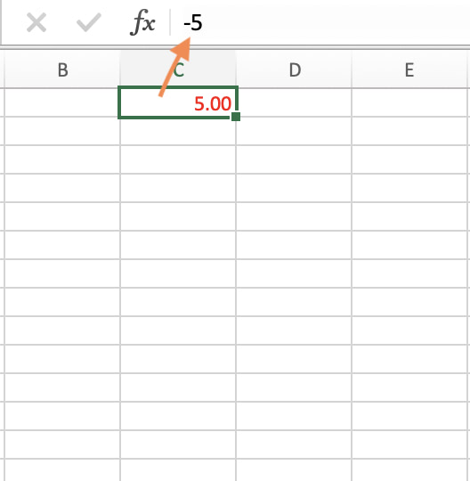
So, let’s say, we have a negative number -5 in C1 cell. If you press Ctrl+1 and select the number formatting to mark the number in red, the result will show a highlighted red text. But, if you click on that C1 cell and look at the formula bar, you notice that the number didn’t change at all.
So, what’s the rule behind this?
We will talk about this rule after we get to know how to actually make negative numbers red in Excel?
Here are the steps to make negative numbers red in Excel using number formatting:
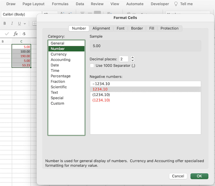
Select the cells you want to highlight. Click on Ctrl+1 to open the Format cells dialog box. Select the Number category list from the Number Tab and click on the red color text in the ‘Negative Numbers’ option. Click OK.
By saving the changes, you will notice that the negative numbers from the selected cells are marked as red texts. With similar steps, you can also add a bracket to the negative number.
But here’s the catch.
Look at the numbers that got highlighted. They all converted into positive numbers, right?
Remember, we told you that the in-built number formatting in Excel is like a disguise that you apply to the cell. Although the red text seems visually positive, it is actually negative by nature.
Now, let’s try a different method. We will use a custom number formatting using the built-in templates.
Use Custom Number Formatting To Display Negative Numbers in Red Color
Custom Number formatting allows you to control how numbers are displayed in cells. So, let’s say you want to fill the cell containing the negative number in red instead of changing the text color. In that case, you can modify the formatting accordingly.
To create custom number formats in Excel, you must use a combination of symbols, placeholders, and special characters. Let’s get to know the basics of custom formatting.
Basics of Custom Number Formatting
Custom number formatting involves specifying a code that tells Excel how to display the data within a cell.
Here’s a complete breakdown of the symbols and characters you see while opening the custom section:
| Common Formatting Elements | Description |
| 0 (zero) | Zero acts as a placeholder for a digit. If a digit is present in the number, it will be displayed. If not, a zero will be displayed in its place. |
| # (Hash / pound) | Unlike the zero, if there’s no digit in that position, Excel will leave it blank. |
| . (Period / Decimal) | Specifies where the decimal point should appear |
| ; (Semicolon) | Creates a separation for positive, negative, zero, and texts. |
| , (Comma) | Adds a thousands separator. |
| / (Slash) | Adds a date separator |
| “ (Double Quote) | Used to include literal characters in the format |
Example: So what does #,##0;-#,##0; 0; @ mean?
The rule is simple. The first part before the first semicolon indicates how you want the positive number to be shown. The second part before the second semicolon shows how the negative number should be shown. Similarly, the rest two parts indicate how you want the zero values and text values to be shown.
So, why should you be using custom number formatting?
It’s because, with normal number formatting, your negative numbers will be visually positive. It might be a problem for some users to cope up with. The solution is to use custom formatting to keep the negative sign intact and also mark the text as red.
Now, you might ask:
How to use the custom number formatting to turn negative numbers red?
Here are the steps to turn negative numbers red:
- Select the range of cells and open the number formatting tab using the keyboard shortcut Ctrl+1.
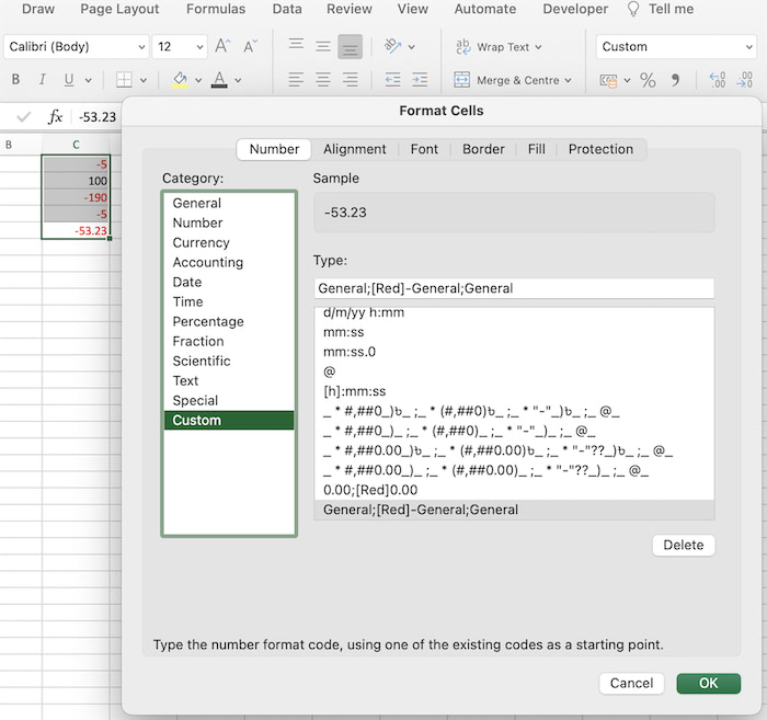
- Navigate to the Custom section and type General;[Red]-General;General.
- Click OK to apply the changes.
Note: If you want to show the negative numbers in brackets, then change the formula to General;[Red]-(General);General and click on OK.
Remember that the formula will be saved on the spreadsheet so that you don’t have to type the code multiple times.
How To Use Conditional Formatting to Show Negative Numbers in Red
Conditional Formatting in Excel is a feature that allows you to apply specific formatting styles to cells or ranges based on certain conditions. The best part about this feature is that conditional formatting doesn’t modify the actual cell values; it only changes the way the data is presented.
So, how can you utilize this feature?
Follow the steps below to use conditional formatting to highlight negative numbers in Red:
- Select the cells containing the values and go to Home Tab.
- Navigate to Conditional Formatting > Highlight Cells Rules > Less Than.
- Type 0 (zero) and modify the colors accordingly.
- Click OK to apply changes.
So, you might ask:
How to make negative numbers red in Excel for Mac?
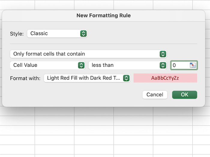
For Mac Users, once you go to conditional formatting > Highlight Cell Rules > Less Than option, a new formatting rule box will appear. Select the classic style and type 0 in the cell value less than the box. Select the formatting options (you can customize the formatting) and press OK.
Use VBA To Highlight Negative Cells Value in Red
Visual Basic Editor is used to simplifying the tasks in Excel. If you are a beginner, just copy and paste the following code:
Sub NegativeNumberAsRed()
Dim cells As range
For Each cells In Selection
If cells.Value < 0 Then
cells.Font.Color = vbRed
Else
cells.Font.Color = vbBlack
End If
Next cells
End Sub
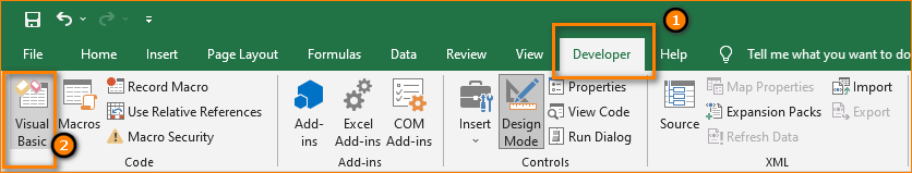
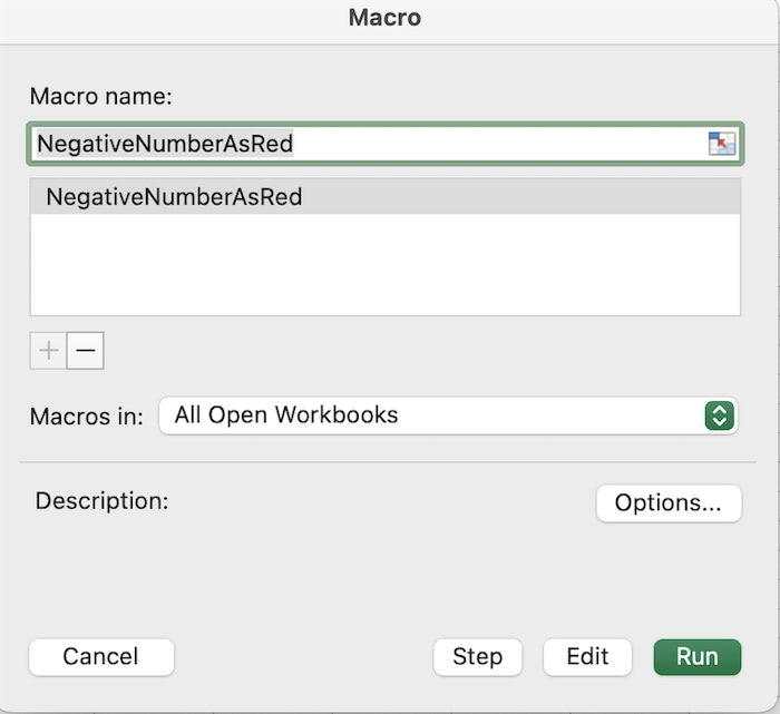
Copy the code. Go to the Developer Tab and click on the Visual Basic Option. Insert a new module and paste the code. Save and Run the code using F5. The moment you return to the Excel spreadsheet, you will see that the negative values are highlighted in red color.
Frequently Asked Questions
Question: How to change the color of negative numbers in Excel?
Answer: You can change the color of negative numbers in an Excel dataset by using both Conditional Formatting and Number Formatting. Select the dataset and press Ctrl+1 to open up the format dialog box. Go to the Number Category and select the red marked text for negative numbers.
Question: How to color positive and negative numbers in Excel?
Answer: To color both positive and negative values in Excel, the easiest way is to use the Conditional Formatting feature. You can add a new rule and customize it accordingly. The second option is using a VBA code. A VBA Code always saves time if you know about Visual Basic and how to create a code.
Question: How to format negative numbers in Excel?
Answer: To format numbers in Excel, use the customizable format from the formatting dialog box. Use Ctrl+1 (for Windows users) or Cmd+1 (for mac users) to open the box and format the values according to the in-built templates.
Question: How to make cells green or red in Excel?
Answer: You can use the 2-scale color formatting from the conditional formatting tab. Ensure that the rule you set contains both the conditions to make cells red and green accordingly.
Conclusion
There are three ways to make negative numbers red or any color you want in Excel. The methods are-
- Conditional Formatting
- Custom Number Formatting
- Application of a VBA code
We find using the conditional formatting very helpful because you can add rules and format the numbers at the same time. It’s like hitting two birds with a single stone.

