
Imagine you are a high school teacher, and you are in charge of organizing a field trip for your students. You have received a mile long list who have signed up for the trip, along with their parent’s names and phone numbers.
As the trip day approaches, you realize that you need to send text messages to the parents to confirm the pickup and drop-off times. Unfortunately, the area code of the numbers is enveloped with parentheses, making it difficult to sort the data quickly. You don’t have time to remove the parentheses from each phone number manually.
To avoid such a situation, it’s better to learn the smart technique in advance so that you don’t hit rock bottom.
Remove Parenthesis Symbol in Excel – 5 Simple Ways
By removing brackets, you can simplify your formulas, making it easier to maintain and update your spreadsheet in the future. In this tutorial, I will show you how to remove parentheses from phone numbers in excel considering the situation mentioned in the introduction.
So, here are the ways you can remove parentheses in Excel:
Method 1: Insert the SUBSTITUTION Function
The SUBSTITUTE function in Microsoft Excel allows you to replace a specific text with another text. It has the following syntax:
Here, the text string indicates the specific data to be searched and replaced.
old_text: The word, symbol, number, or data to be searched.
new_text: The string to replace the old text.
instance_number (optional): The instance of old_text to replace. If you omit this argument or if you specify a value of 0, all occurrences of old_text will be replaced.
In my dataset, the area code of the numbers is enveloped in brackets. So, I have to delete them to make the data more neat.
I will be using the formula =SUBSTITUTE(C5,”(“,””). The formula represents replacement of every occurrence of the text “(“ with an empty string in the contents of cell C5. Next is using =SUBSTITUTE(D5,”)”,””). 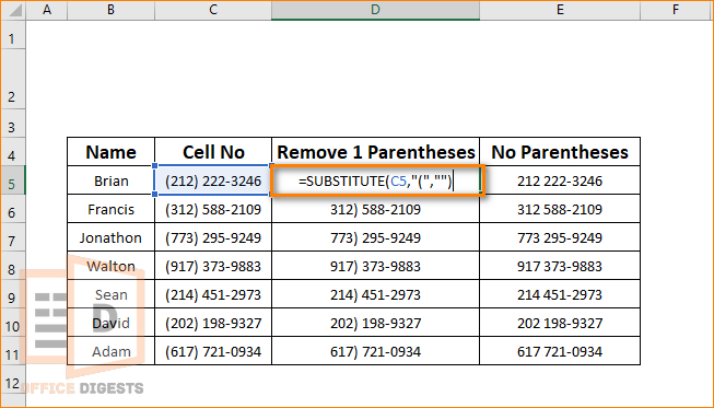
By now, you understood that this is a two-step process. In other words, if you use the SUBSTITUTE function, you have to use the formula twice for a decent outcome.
Method 2: Use the Find and Replace Feature
This method is also a two-step process.
Do you still remember the mnemonic (BODMAS) we used to remember the order of operations in mathematics?
BODMAS is an acronym that stands for Brackets, Orders (such as powers and square roots), Division and Multiplication, and Addition and Subtraction. It specifies the sequence in which you should perform the calculation to get the correct answer to a mathematical expression.
In Microsoft Excel, it’s generally a good practice to remove unnecessary angular brackets to make your data easier to read, understand, and maintain. You can use the Find and Replace Option to do so.
You may ask:
How to access Find and Replace in Excel?
Here’s how:
- Select the range of cells where you want to search for the bracket.
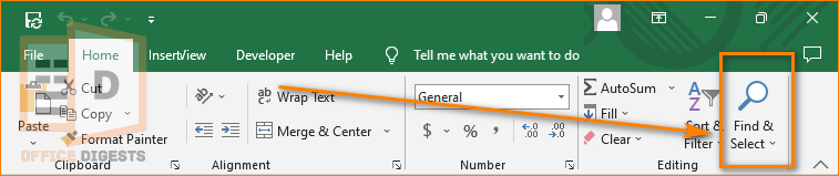
- Go to the Home Tab and click on Find & Select.

- Press on the drop-down menu and select the Replace option. Alternatively, you can use the Keyboard Shortcut (Ctrl+H).
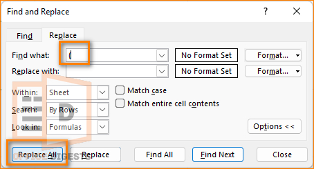
- Type the starting bracket ( in the Find What box and click on Replace All. Similarly, type the closing bracket ) and select Replace All. In both cases, keep the Replace with box empty.

How to Remove Parenthesis With Text Using The Find and Replace Feature
Select the range of cells you want your operation to take place. Type (*) in the Find What Box and keep the Replace With box empty. Select the Replace All Option to delete brackets with text. The asterisk symbol (*) is used to denote wildcard entry. 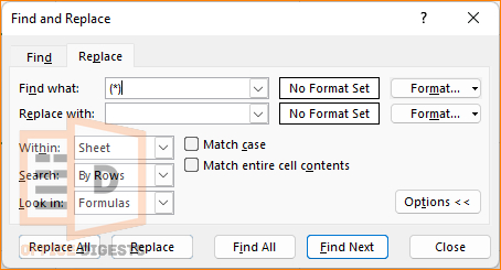
Method 3: Embed a VBA Code
Using VBA Codes is the fastest way to delete brackets from texts or phone numbers. To do so, first you have to enable the Visual Basic option in Excel. Then go to the Developer Tab > Visual Basic Option > Insert Module. Select the Module 1 and paste the following code.
Option Explicit
Sub DelParentheses()
Cells.Select
Selection.Replace What:="(", Replacement:="", LookAt:=xlPart, _
SearchOrder:=xlByRows, MatchCase:=False, SearchFormat:=False, _
ReplaceFormat:=False
Selection.Replace What:=")", Replacement:="", LookAt:=xlPart, _
SearchOrder:=xlByRows, MatchCase:=False, SearchFormat:=False, _
ReplaceFormat:=False
End Sub
Run the module using the F5 option or clicking the Run Sub/UserForm button. Go to the Excel Spreadsheet and see the magic.
But, here’s what you need to know.
While using macros, many users face a problem where they see that the number they type in is pre-formatted to a text. To solve this issue you have to use another vba code to convert text to number format.
Method 4: Combine the LEFT And FIND Functions Together
The LEFT function in Microsoft Excel returns a specified number of characters from the beginning of a string of text. Let’s say I have two words, “Happy Halloween”.
The syntax of LEFT Function is =LEFT(text, [number of characters]). So, if I use the formula =LEFT(A1, 5), the result will be Happy.
Again, the FIND Function is to find a specific text in that range of cells. If Excel doesn’t find the text, the function returns a #VALUE! Error.
I write below the formula I will use here and it’s a one-step process.
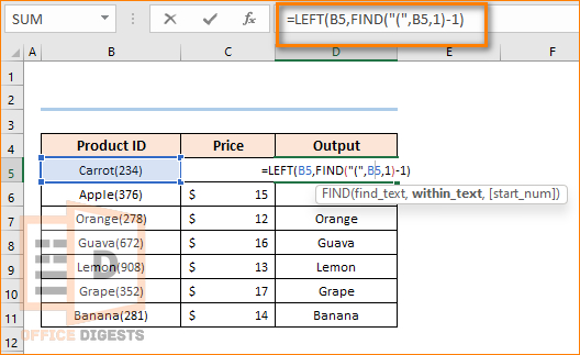
Explanation of the Formula
So, what’s happening here is the first argument, “(“, is the character to search for, and the second argument, B5, is the cell containing the text. The third argument, 1, is the starting position for the search, which is set to 1 so that the search starts from the beginning of the String. After that, the result of the FIND function is then subtracted by the value 1 to get the position just before the first occurrence of the character “(“.
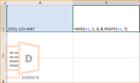
Method 5: Apply The RIGHT And MID Function
Suppose you have a column of phone numbers in the format (555) 123-4567. To remove the parentheses and keep only the digits, you could use the combination of both MID and RIGHT functions.
The RIGHT function is used to extract the last seven digits, and concatenate them with the MID function to extract the first three digits.
So, the formula stands out to be:
Change the variable according to your preference. For example, select a different active cell to apply the formula.
FAQ
Q: What are parentheses in Excel?
A: Parentheses are a pair of symbols used to group mathematical operations. It also indicates the order in which you should perform the calculations. For Example: Consider the formula, =(2+3)*4. The parentheses here indicate that the addition of 2 and 3 needs to be performed first. And the result 5 should then be multiplied by 4. So, the answer will be 20.
Q: How Excel calculates more than one parenthesis?
A: When there are multiple sets of parentheses in a formula, Excel will perform the calculations inside the innermost set of parentheses first, and then work outward. For Example: Consider the formula, =(2+3)*(4+5). Excel will first perform the calculation inside the brackets, resulting in 5 and 9, respectively. Then it will multiply the two results 5 and 9 to provide the conclusive answer 45.
Final Words
Now, if you ever run into a situation of removing the round brackets off the numbers, you can easily amaze others by not stressing a lot. Use any of the five methods that suit you as all the methods are 100% working.

