Use Greater Than or Equal To Symbol in Excel [4 Examples]

Suppose you are a schoolteacher and you are making a grading sheet of your class.

In that worksheet, you want to use a formula to calculate the grades based on the scores. Also, you want to highlight the ones who scored greater than or equal to a certain percentage. In this situation, you will need some mathematical operators like the ≥ symbol.

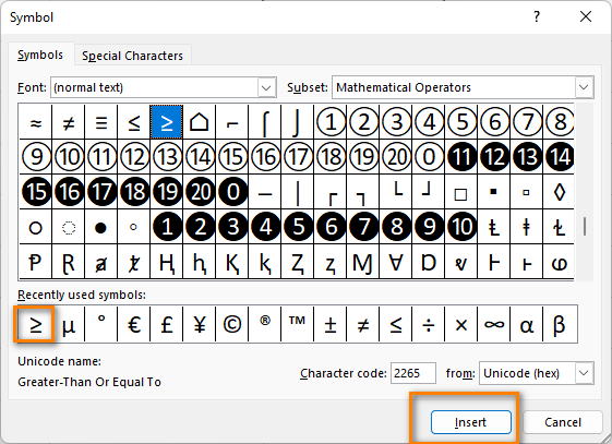
How did I insert the symbol? Well, in MS Word, it’s really easy to insert special characters. However, there are a few methods to insert the greater than or equal sign in Excel.

Stay with me to learn more about these steps.

How is the Greater Than or Equal To Symbol Written in Excel?

In Excel, you can’t use the ≥ symbol in this format in a formula. You have to insert the greater than (>) sign followed by an equal to (=) symbol. However, if you are not generating any equation or formula in a worksheet, go to the Insert Tab > Symbol > Maths Symbols to insert the ≥ sign in the active cell.

For Example, look at the dataset in the following image.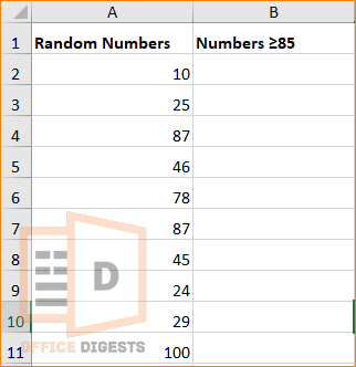

I have ten numerical data starting from 10 and ending up at 100 and I want to find out which numbers are greater than 85. For this, I am using A2 as my reference cell. Next, I am using an equal to (=) sign to start my formula. The formula turns out to be =A2>=85.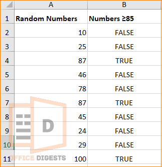

And the returned result is in TRUE or FALSE. By navigating through the TRUE values, I am figuring out which numbers are greater than or equal to 85 in my dataset. You can also use the filter function to sort the data.

You can use this greater than and equal to operator (>=) along with some Excel functions like the SUMIF, and COUNTIF Functions.

Relational Operators in Excel

Relational operators are such symbols used to compare between two datasets. There are six relational operators that give a Boolean value.

Consider a dataset of A1, A2, A3, A4, A5 having values 30, 40, 50, 60, and 70 respectively. Now, follow the example and the result based on the criteria.

Relational Operation	Symbol	Example	Result
Equivalence	=	=A1=23	FALSE
Less Than	<	=A5<100	TRUE
Less than or equal to	<=	=A2<=20	FALSE
Greater than	>	=A4>50	TRUE
Greater than or equal to	>=	=A2>=30	TRUE
Not Equal to	<>	=A5<>60	TRUE

When Should Relational Operators be used in Excel?

Here are some situations where you should be using the relational operators: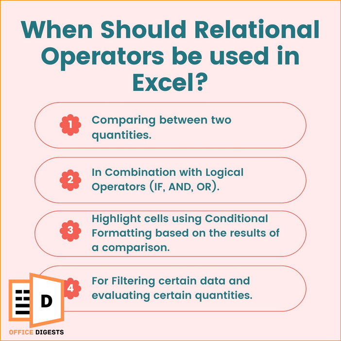

Comparing between two quantities.
In Combination with Logical Operators (IF, AND, OR).
Highlight cells using Conditional Formatting based on the results of a comparison.
For Filtering certain data and evaluating certain quantities.
To compare two values with a third-one of the same data type.

How To Use The Greater Than or Equal To Operator in Excel

You can use the greater than operator in combination with many functions in Excel. For Example, the IF function, COUNTIF Function, and also the SUMIF function. Let’s elaborately discuss it by providing some great examples.

Example 1: Use the Normal Cell Reference Technique

Like I said, you are a schoolteacher and want to make a grade sheet for your class. Look at the image attached below.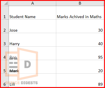

I have a list of students’ names along with their marks. Let’s say you want to find out if any of your students scored above 85. For that, type in the formula below and Press Enter.

=B2>85

The value will return a result as TRUE If any of your students scored above 85 marks. Use the Autofill Function to drag the formula to the desired range of cells.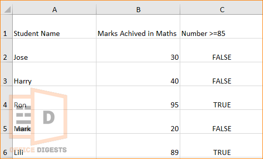

Now let’s focus on another condition where you want to grade the numbers achieved by your students.

Example 2: Use the IF Function For One or More Criteria

Suppose, in the same mark sheet, you want to find out who failed and who passed the test. Let’s say the minimum threshold is 40. You are considering below 40 marks as F Grade.

Now, type the IF Function on Cell C2. Then for the logical_test, I am going to set the criteria as B2>=40. If the condition is satisfied, then Excel will show the word “PASS”. If not, then “FAIL”.

So, the formula is:

=IF(B2>=40, “PASS”, “FAIL”)

Press Enter and use the autofill handle to set the formula up to the desired range.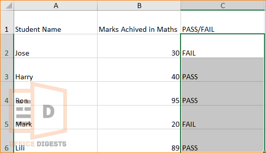

Example 3: Apply The COUNTIF Function

This section is for counting the number of students who passed. If you have a large dataset and you graded them using the IF Function, it’s now time to count the total number of students who passed or failed.

I have made a complete guide for the COUNTIF cell not blank formula in Excel. You can check it out for a detailed explanation of this function.

Now, with the same dataset, execute the COUNTIF Function. You will need a range and a criterion to generate the formula. For the range, I am selecting the cells B2:B6, and my criteria is to find the number of students who got marks above 40.

So, my formula is:

=COUNTIF(B2:B6, “>=40”)

number-of-students-passed-using-countif-function

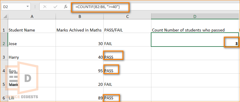
Press Enter and now you know how many students passed in your exam. You can also use the less than or equal to operator to find the number of students who failed the exam. In that case, the formula will be:

=COUNTIF(B2:B6, “<=40”)

Note: Enter a space after selecting the range of cells or before applying the criteria.

Example 4: Implement The SUMIF Function in Combination with Greater Than or Equal To Sign

Let’s expand our datasheet. You will see the grades of different subjects for each of your students. If you want to calculate the total number of each student, excluding those marks which are below 40, then move along.

Execute the formula by typing:

=SUMIF(B2:E2,”>=40″)

use-sum-if-to-calculate-total-grade-of-students

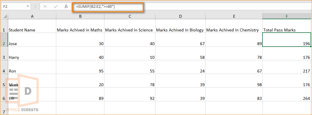
This formula will allow the summation of only the pass marks. Use the Fill Handle to drag the result until desired range. Notice that the marks below 40 are omitted due to the criteria.

Note: Suppose you want to add multiple criteria, like finding a student’s name and adding his mark with one formula. You can use the SUMIFS Function for multiple columns statement.

How To Insert The ≥ Symbol in Excel

Inserting symbols are easy and there are many alternatives to do so. Here are four ways to insert ≥ symbol in Excel:

Use the Symbol Command. Go to Insert Tab > Symbol > Add the required symbol.
Apply the Keyboard Shortcut. For Mac users, Hold the Option button and Press the > symbol. And use ALT+242 if you are a Windows user.
Use the Equation Command. Go to Insert > Equation > Add the symbol > Copy it and paste to the required cell.
Google the greater than or equal to symbol and copy the sign. Paste it on the required cell.

Final Words

Whether you are looking to sort data, create formulas, or highlight certain cells, the greater than and equal to (>=) operator can be used to help you achieve your goals efficiently. You can compare values and perform conditional formatting based on that comparison swiftly.