
If you want to compare two big columns on different sheets, but you have no idea how to do that, then you are in the right place. In this article, we will show you some of the best ways through which you can easily use the VLOOKUP formula to compare two columns in different sheets.
There are times when you will need to compare data from two separate lists in order to determine what things are missing from one of the lists and what info is included in both lists. Different methods of comparison exist, and the approach that is most appropriate for your needs will depend on those needs.
But we all know that using the VLOOKUP function is the easiest and most effective way to do that. So, keep reading this post until the end to learn in detail.
How To Use VLOOKUP Formula To Compare Two Columns in Different Sheets
To demonstrate the whole process, we structured an Excel file that contains two sheets. One is for the 100 most frequently given names for boy newborns children throughout the past 100 years, from the year 1918 to 2017, which are included in the First spreadsheet.
In addition, Sheet 2 has the top 100 most popular boys given names in the United States.
So, let’s look at the names of the Sheet 1 worksheets in comparison to the names of the Sheet 2 worksheets.
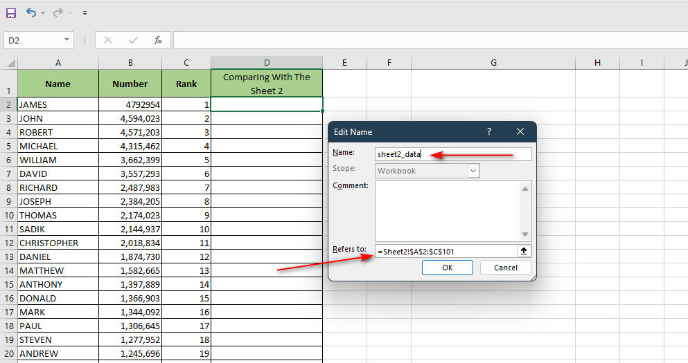
But before we do that, we have to define a formula for the sheet range. To do that:
- Go to the Formulas tab and click on the Define Name
- On the Name field, type sheet2_data
- On the refers to the field, enter: Sheet2!A2:C101
Now, we can just enter sheet2_data on the range_lookup part of the formula.
Hence, follow the steps below to do the main task:
- Insert a new column named Comparing with The Sheet 2 next to the Rank column in the Sheet 1.
- Now enter the below-given formula in cell D2: =VLOOKUP(A2, Sheet2!A2:C101, 1, FALSE)
- Once you enter the formula in cell D2, hit the Enter button on your keyboard, and you are done.
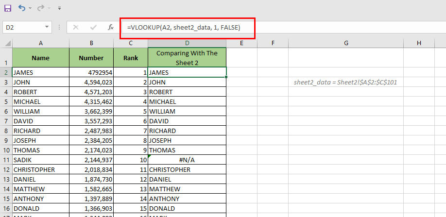
Now you will see that the name James appeared on the D2 cell. And this name appeared here because this name is also available in Sheet 2.
So, in order to copy this formula into the below-remaining cells, double click on the Fill handle option, which is located on the right bottom corner of the D2 cell.
Did You Know? You can also use the VLOOKUP function to return all matches in an Excel worksheet.
How To Deal With The #N/A Errors With IFERROR and VLOOKUP combo
If you have done the above steps carefully, then you will notice that there are some #N/A errors that appear in the column. If you want, you can leave that as it is. But, in my opinion, when there is a great way to handle this eyesore, then why should I not fix it?
You can easily fix the #N/A errors in Excel by using the IFERROR function. It is mainly used to treat the errors that come in almost all kinds of situations.
How does IFERROR Formula work?
You must be knowledgeable about the IFERROR excel function in order to comprehend this method. So, the syntax of this formula is:
=IFERROR(value, value_if_error)
Here we can see the arguments:
Value: We have used the VLOOKUP formula as the value of the IFERROR function. To summarize: If no error occurs, the result of the VLOOKUP equation will be equal to the result of IFERROR’s function.
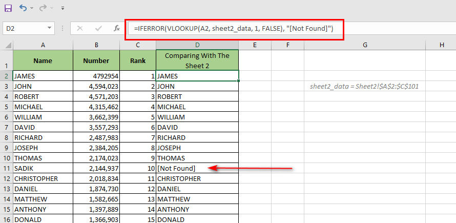
Value_if_error: As the value_if_error parameter, we’ve entered the string [Not Found] as the value to check for. Consequently, if the IFERROR function detects an error in a cell, it will display the string [Not Found] if an error is discovered.
So, now that we understand how this formula works, let’s move on to the main steps where we can actually know how to fix the #N/A errors in Excel:
- Open the spreadsheet and enter the formula given below in cell D2: =IFERROR(VLOOKUP(A2, sheet2_data, 1, FALSE), “[Not Found]”)
- Now double click on the Fill Handle option to copy and paste the formula on the remaining cells.
Fix The #N/A Error By Using IF, ISNA, and VLOOKUP Combo
Although we can use the IFERROR function as described in the above section, there is also another way to deal with the #N/A errors in Excel. And that way is to use the IF, ISNA, and VLOOKUP combo to handle the #N/A errors.
So, to do that, follow the steps below:
- Open the file and enter the following formula in cell D2: =IF(ISNA(VLOOKUP(A2, sheet2_data, 1, FALSE)), “Not Matched”, “Matched”)
- The Matched string text will appear as soon as you hit the Enter button on your keyboard.
- Now, double-click on the Fill Handle option to copy and paste the formula on the remaining cells.
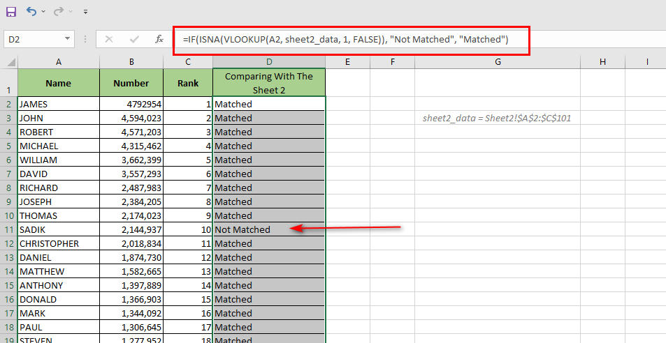
After you have done that, the string Not Matched text will appear on the cells which were showing errors. Isn’t that a fantastic way to handle the errors?
Now, are you curious about how this formula works? Then keep reading the below part.
How Does the ISNA Formula Work
To comprehend this formula, you must be familiar with the operation of the IF and ISNA functions.
The following is the syntax for the IF function: =IF(logical_test, value_if_true, value_if_false)
And the following is the syntax for the ISNA function: =ISNA(value)
Let us now analyze the functioning of the following formulas:
Logical_test: Our VLOOKUP value is held in our ISNA function, which has been given to the IF function as the logical_test parameter of the IF function. In the event that the VLOOKUP formula gives a #N/A error, the ISNA function will return the TRUE result.
Value_if_true/false: [Not Matched] is the result returned by the IF function when the logical_test is True. ISNA will yield FALSE if the VLOOKUP function gives a value (i.e., there was no error). This means that False will be returned as the result of the IF function’s logical test parameter. And as we have given the string [Matched], this text will be returned when the logical test is False.
Conclusion
The Vlookup formula does come in handy when it comes to comparing two columns in different sheets. And so, we have given some of the best techniques to use this formula. We hope this article has helped you to know how to use the VLOOKUP formula to compare two columns in different sheets.

