3D interpolation is often needed to estimate the values of a 3D surface from the given data points. It’s useful for spatial, time series, or any other types of 3D data.
Since there’s no built-in 3D interpolation function in Excel, you must use a VBA module for the purpose.
In the following article, we will provide step-by-step instructions on performing 3D interpolation in Excel.
Therefore, let’s begin.

Can you do 3D Interpolation in Microsoft Excel?
Microsoft Excel does not have any default function for interpolation in 2D, 3D, or other dimensions. However 3D interpolation can be done in Excel by writing a custom VBA module.
Interpolation is a method that helps us to evaluate values between known data points. Let’s say you know the value of a function at points (1,1) and (1,2), but you need the function value at the point (1,1.5), which is unknown. By using interpolation, you can find the unknown value.
Interpolation is possible with 2D, 3D, or other higher-dimensional data points. It is often needed in data analysis where we want to find the intermediate data points from the known data points.
Here, we will show you how you can create a 3D Interpolation function in a straightforward procedure.
How to Perform 3D Interpolation in Excel
In Excel, you can perform 3D interpolation by writing a custom VBA module containing the interpolation function. You’ll need the input 3D data points (known or given data), and the target data points (unknown) on which you want to interpolate the values.
You will create a UDF (user-defined function) using a VBA module and then use the newly created function to calculate the interpolation values.
There are many interpolation algorithms. Since we’re dealing with 3D interpolation, we’ll be using the trilinear interpolation for our purpose.
Let’s now create and use the interpolation function in Excel.
Here is the method to 3D Interpolate in Microsoft Excel:
1. Paste the Known Data Points
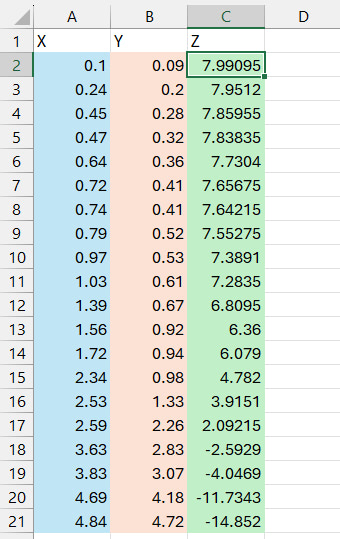
Launch Microsoft Excel and paste the known or given data into the sheet. Since you’re dealing with 3D data, paste the x, y, and z-values in their separate columns. 
2. Create a Module with VBA
Press Alt+F11 to open Visual Basic Editor. Click on Insert > Module and paste the following code: choose-module-in-visual-basic
Function INTERPOLATE3D(x As Double, y As Double, sourceRange As Range) As Double
    Dim xValues As Variant
    Dim yValues As Variant
    Dim zValues As Variant
    Dim xIndex As Integer
    Dim yIndex As Integer
    ' Assuming sourceRange is structured with x-values in the first column, y-values in the second column, and z-values in the third column
    xValues = sourceRange.Columns(1).Value
    yValues = sourceRange.Columns(2).Value
    zValues = sourceRange.Columns(3).Value
    ' Find the index of x in xValues
    For xIndex = 1 To UBound(xValues, 1) - 1
        If x >= xValues(xIndex, 1) And x <= xValues(xIndex + 1, 1) Then
            Exit For
        End If
    Next xIndex
    If xIndex = UBound(xValues, 1) Then xIndex = UBound(xValues, 1) - 1
    ' Find the index of y in yValues
    For yIndex = 1 To UBound(yValues, 1) - 1
        If y >= yValues(yIndex, 1) And y <= yValues(yIndex + 1, 1) Then
            Exit For
        End If
    Next yIndex
    If yIndex = UBound(yValues, 1) Then yIndex = UBound(yValues, 1) - 1
    ' interpolation
    Dim xFraction As Double, yFraction As Double
    xFraction = (x - xValues(xIndex, 1)) / (xValues(xIndex + 1, 1) - xValues(xIndex, 1))
    yFraction = (y - yValues(yIndex, 1)) / (yValues(yIndex + 1, 1) - yValues(yIndex, 1))
    Dim c00 As Double, c01 As Double, c10 As Double, c11 As Double
    c00 = zValues(xIndex, 1)
    c01 = zValues(xIndex, 1)
    c10 = zValues(xIndex + 1, 1)
    c11 = zValues(xIndex + 1, 1)
    Dim z0 As Double, z1 As Double
    z0 = c00 * (1 - yFraction) + c10 * yFraction
    z1 = c01 * (1 - yFraction) + c11 * yFraction
    INTERPOLATE3D = z0 + (z1 - z0) * xFraction
End Function
Press Ctrl+S to save and exit the Visual Basic window.
You have successfully created the INTERPOLATE3D function. Now you will use this function to interpolate intermediate data points.
3. Paste the Target Data Points and Plot the Surface
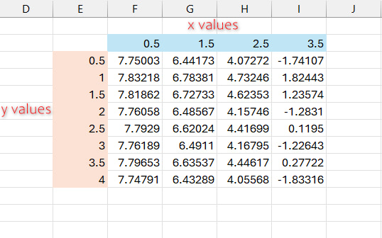
First, you need to put the target data points into the sheet. Here, I have taken the x-values horizontally and the y-values vertically to form a grid. But you can put the values along the columns as well. 
Our function has the following syntax:
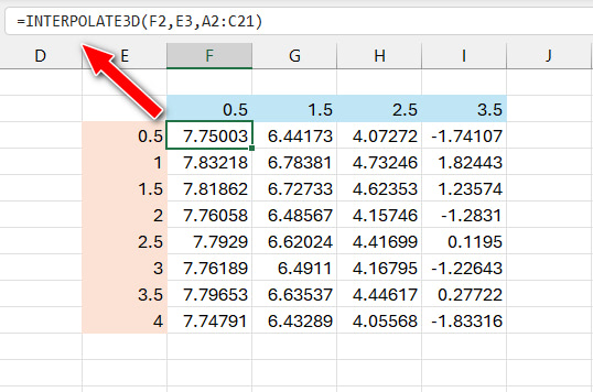
To use the function, select a cell and type the following in the formula bar:

Here, F2 and E3 reference the x and y-values of the target data point which we want to interpolate, and A2:C21 is the range of given data points (x, y, and z values).
You can use the INTERPOLATE3D function similarly to interpolate the remaining data points. You just need to change the x and y-value cell references (the first and second arguments in our function).
To create the surface plot from the interpolated values:
- Select the interpolated values.
- Click on the Insert tab and select Recommended Charts.
- Select Surface from the left ribbon and click OK.
So, the 3D graph is ready with interpolation in Excel.
Final Words
3D interpolation in Microsoft Excel is a powerful technique that allows you to estimate intermediate values on surfaces using some known data points in three dimensions.
By employing this method, you can fill in missing values, and reveal the underlying patterns in your data.


