When you are dealing with a large amount of data, sorting data automatically in Excel can be extremely beneficial. Excel does not have a built-in function for automatically sorting your data. But don’t worry; in this article, we are going to show you some of the best ways through which you can easily auto-sort when data is entered in an Excel spreadsheet.
There are several ways to sort data automatically in Excel. For example, by using the SORT function, using the VLOOKUP function, or using VBA. We will learn these three methods to sort data in our Excel spreadsheet.
So, keep reading this post until the end to learn in detail.
How to Auto Sort When Data Is Entered In Excel
As we have already told you before, we will share the three most effective ways to sort data automatically in Excel. Those methods are:
1. Use the SORT Function To Auto Sort Data In Excel
You can use the SORT function to organize your data set so that it is presented to you in either ascending or descending order. However, there are three kinds of auto sorting data ways available in Excel. The three ways we will talk about now are: Ascending order, Descending order, and auto sorting multiple columns.
Note: Keep in mind that the SORT function is now only accessible in Microsoft 365 and Excel 2021, which are the latest versions of the product, because Dynamic Array formulae are Not Supported in Excel 2019, and Excel 2016. So, the SORT function is not accessible in these versions of the spreadsheet software program.
Hence, now let’s move on to the main topic of our article:
i. Automatically Sort Data in Ascending Order
Assume that we have a worksheet containing two columns, one is the Product Name, and another one is the Stock. Now, we want to sort the table in ascending order.
But, how does the formula work?
The Syntax of the SORT formula is:
=SORT(array,[sort_index],[sort_order],[by_col])
Here we can see what the arguments imply:
Array: Array refers to the data range you’re working with (B5:C14).
[sort_index]: A number specifying the row or column that should be sorted in the database.
[sort_order]: A number defining the preferred sort order; 1 indicates ascending order (the default), while -1 indicates descending order.
[by_col]: It’s totally optional like the above two arguments. But we will need the above two arguments, while this one is not required. But, you should at least know that it is a logical value specifying the intended sort order; for example, FALSE to sort by row (the default) and TRUE to sort by column (the alternative).
Now, to sort automatically, follow the steps below:
- Open the spreadsheet and copy and paste the whole table beside it.
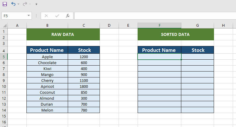
- Then enter the following formula on the first cell of the product name column, which is, in our case, cell F5: =SORT(B5:C14,2,1)
- Click on the Enter button on your keyboard after entering the above formula.
We are now able to get the data out in ascending order since it had been auto-sorted. If you make a modification to any of the values, the data will automatically sort according to the new value.
ii. Automatically Sort Data in Descending Order
In this step, we will sort the data in descending order. To do that, follow the steps below:
- Open the spreadsheet and copy and paste the whole table, just like the previous method.
- Now enter the following formula in cell F5: =SORT(B5:C14,2,-1)
- Click on the Enter button on your keyboard after entering the above formula.
And now, we have got our auto sorted excel data in descending order.
But, you may think about whether this sorting is auto or not.
Don’t worry; it is auto-sorted. To check whether it is or not, we are going to change the value of KIWI from 800 to 3000. Once we pressed the enter button on our keyboard, the position of KIWI changed and raised to the first row.
In this way, you can easily auto-sort data in descending order in Excel.
iii. Automatically Sort Data In Multiple Columns When Data Is Entered
Now that we know how to auto sort data in ascending and descending order in an Excel spreadsheet, it’s time to know how to auto sort data in multiple columns when some data is entered.
We now wish to automatically sort numerous columns in a worksheet. Let’s take these steps one by one:
- Open the spreadsheet and copy and paste the whole table, just like the previous method.
- Now enter the following formula in cell F5: =SORT(B5:C14,{1,2},{1,1})
- Click on the Enter button on your keyboard after entering the above formula.
And now, we have got our auto sorted data in multiple columns when data is entered.
Now, to check whether this table is auto sorted or not, change one of the names, like replace Avocado to chocolate, and you will see the data will be auto sorted.
2. Use the VLOOKUP Function To Auto Sort Data In Excel
If you are so unfortunate as me, and you are using Microsoft Excel 2016 or earlier, then you won’t be able to use any of the previous methods I described above. So, what’s the solution? Won’t you be able to sort your data in Excel automatically? Well, the answer is yes, you can.
By using the VLOOKUP function, we can easily auto-sort Excel sheets when data is entered.
Now, for demonstrations, we will use the same data we used for the previous methods. Now, get that table and follow the below steps carefully:
- Open the spreadsheet and insert a new column named Rank beside the Product Name column.
- Now to rank the values in this column, we will use the Rank function, which is: =RANK.EQ(E4,$E$4:$E$13)
- After entering the formula, hit the Enter button and fill down all the below cells by using the Fill Handle option.
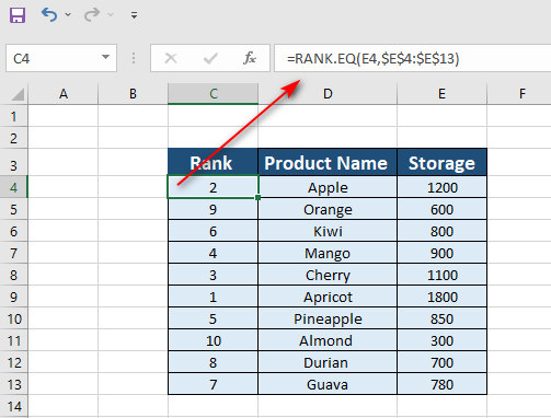
Once you are done, now, the data in this column will be ranked by their values.
Now, just like the previous methods, we copied and pasted the Headings beside the table, do this again in this step.
On the new blank Rank column, enter the number from 1 to 10 consequently.
- On the cell H4, enter the following VLOOKUP formula: =VLOOKUP(G4,C$4:E$13,2,FALSE)
- Hit the enter button on your keyboard.
- Now copy and paste the formula in the below remaining cells by using the Fill Handle
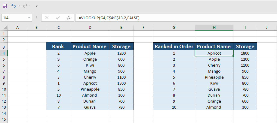
Once you are done following the above steps, you get your auto sorted value according to the lookup_value.
Now, if you want to check whether this table is auto sorted or not, change any values in the main table (table_array) and see if it will instantly affect the ranking of the sorted table.
3. Use VBA To Auto Sort Data In Excel
If you like something complicated, then this method is only for you. In this step, we will make use of the VBA macro in Excel in order to auto our worksheet.
Now, follow the below steps to do that:
- After opening the spreadsheet, open VBA by clicking on the Developer tab and clicking on View Codes.
- Now enter the below-given formula in the blank white box:
Private Sub Worksheet_Change(ByVal Target As Range)
On Error Resume Next
If Not Intersect(Target, Range(“B:B”)) Is Nothing Then
Range(“B1”).Sort Key1:=Range(“B2”), _
Order1:=xlAscending, Header:=xlYes, _
OrderCustom:=1, MatchCase:=False, _
Orientation:=xlTopToBottom
End If
End Sub
In this formula:
B:B indicates that it will automatically sort Column B.
B1 is the first cell of Column B, and so on.
B2: Column B’s second cell is B2.
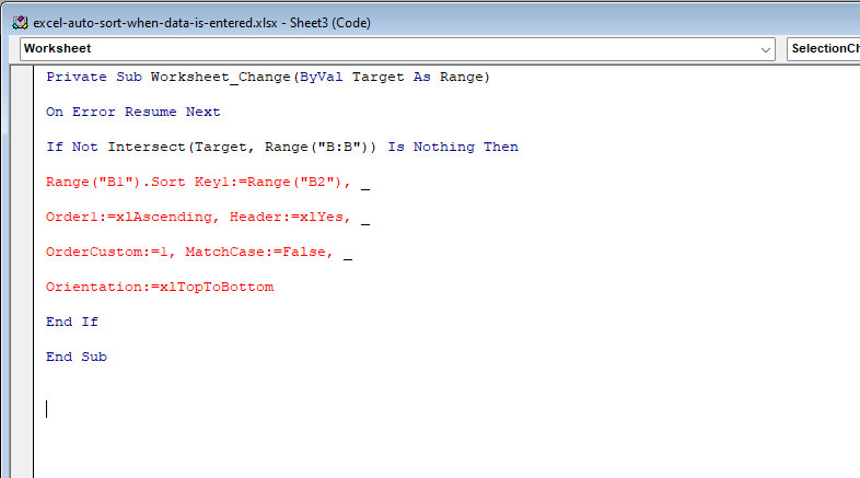
Now, after you have entered the formula in the VBA code, close the window, and you will see that the table has been auto-sorted.
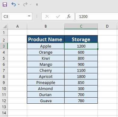
If you now make some changes in the values, the sorting will be done automatically.
And in this way, you can use auto-sort an Excel spreadsheet when data is entered.
Tips and Notes
- The SORT feature is only accessible in the Excel 365 version of the program. Without this particular version of Excel, you will not be able to utilize this feature at all.
- When using the SORT method to automatically sort several columns, the very first column will be auto-sorted first, followed by the other columns. The next column will be sorted once the first column has been sorted, and so on.
- Assuming that the array produced by a SORT function is the final outcome (— for example, not given to the other function), Excel will automatically generate and fill an appropriate-sized range with the sorted data. As a result, make sure you do have enough empty cells below or to the right of the cell in which you input the formula, or else you will get a #SPILL error message.
- When using the VLOOKUP function, keep in mind to Lock the “Table Array” by pressing the F4 key when doing so.
- When you utilize the VBA code, you must replace the value from the spreadsheet in the code with your own value from your spreadsheet.
Also, the results are updated automatically in response to changes in the underlying data. But, the array provided to the function does not immediately expand to cover additional items that are placed outside of the referred array, as is the case with the linked array.
So, such elements must be included in your formula, which means either updating the array references in your formula or creating a table from the source range.
Conclusion
Sorting the data is very useful in Excel. And if it becomes automatic, then things get even better. So, in this post, we showed some of the best ways to auto-sort data when some data is entered in Excel. We hope this article has helped you to know how you can easily auto-sort when data is entered in an Excel spreadsheet.


