How To Use Excel Index & Match With Multiple Criteria [2023]

To solve complex lookup problems, you might want to use the VLOOKUP function instead.

But here’s the catch.

The Vlookup formula doesn’t work if your lookup problem is too complex. That’s where the INDEX and MATCH Functions come to the rescue.

No matter how complex your lookup problem is, you can use INDEX MATCH Functions to get your job done.

In this tutorial, we will guide you through the right way of using the INDEX MATCH functions based on multiple criteria.

Is INDEX and MATCH Better than VLOOKUP?

The answer depends on the criteria of the data. But, in most cases, VLOOKUP is problematic. INDEX and MATCH Functions aren’t VLOOKUP but it is much better than VLOOKUP. Because, in most of the cases, VLOOKUP is not working if your lookup data is complex.

However, you can run the INDEX and MATCH functions together and solve critical problems based on multiple criteria.

INDEX and MATCH are generally faster than VLOOKUP for large datasets, especially if you are looking up values across multiple columns.

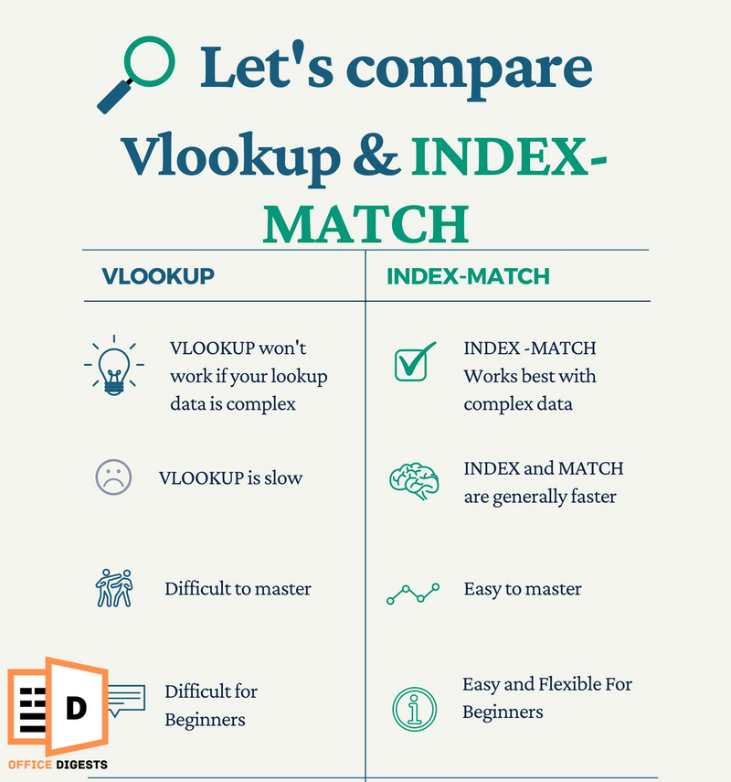
Personally, we use the INDEX functions often. It’s not that easy to master. It’s just that you have to push yourself in the beginning to practice using this LOOKUP function.

Before moving to the complex problems, we should first know how the INDEX and MATCH Functions work, alone.

How Does the INDEX Function Work in Excel?

The INDEX function in Excel is used to return a value from an array, based on the row and column number provided.

Think of this function as a GPS. For the GPS to run, you need to create a map. And that map is the INDEX Function.

The basic syntax of the INDEX Function is:

The INDEX Function contains three arguments. Out of which two are the required ones. The column number argument is the optional one. As you can see, it is inside a square bracket.

The array argument required here is the map you need for the INDEX Function to work. It should contain the answer you are looking for.

In some cases, you may need to extend the map (that is, the range of the lookup array).

The next two arguments are to specify the row and column numbers for the INDEX function to look across for the result.

So, it’s basically like the longitude and latitude of the map. If you move outside of the map, you will get error values, exactly like the #REF! Error when you use VLOOKUP to return all matches.

How Does the MATCH Function Work?

MATCH function is a function that acts as a helping hand for the INDEX function. MATCH Function returns a number to the INDEX if you want to automate the row and column number.

Yes, you do have the COUNTA, ROW, COLUMN functions to use as an argument for the INDEX Function. But, there’s only a handful of cases where you will be using that.

So, the best suited function that works in harmony with the INDEX Function is the MATCH Function.

Here’s the syntax for the MATCH Function:

The first argument is what we are looking for. It may be a text or a number string. Next is the lookup_array. That is, where is the MATCH function going to find the value?

One thing to note here is that,

The MATCH Function is a one-way street. You cannot add a whole range of data from two or more columns or rows. The appropriate example would be using the lookup_array as A2:A10, instead of A2:B10.

The third argument is the match type, whether we want the exact match, less than, or greater than a number in Excel.

In most cases, we need the number 0 to find the exact match.

Final Result?

Well, Excel will return a number instead of a specific text. Suppose the answer is 7. This means that the position of the value we are looking for is in the 7th position in that particular row or column.

Now, let’s use the INDEX and MATCH Functions together.

How To Use The INDEX and MATCH Functions Based on Multiple Criteria

To make the two functions work in harmony, you have to focus on the aim of the formula. Of course, we want to use these functions for a complex lookup problem.

And to solve this problem, we need the INDEX function first. After that, we want the MATCH function to return a value to the INDEX function.

Well, that’s the basics for sure.

But, how do you use index and match combined?

Now, let’s take an example and the detailed process to use these two functions together.

Here are the steps to use the INDEX and MATCH functions together with multiple criteria:

1. Ensure if the Dataset is INDEX-MATCH Compatible

The first and foremost problem we see is that users try to forcefully incorporate the INDEX-MATCH functions even if it’s not compatible.

Maybe a simple COUNTA would’ve solved the problem. Or even a XLOOKUP function.

The best thing we can suggest to you is to first identify your goals.

Ask yourself:

• Is this problem related to looking for a value?
• Does the dataset have data validation?
• Is the Array Length and Width Same?

If all the answers are yes, then proceed…

Let’s look at a general dataset by creating a real-life lookup problem.

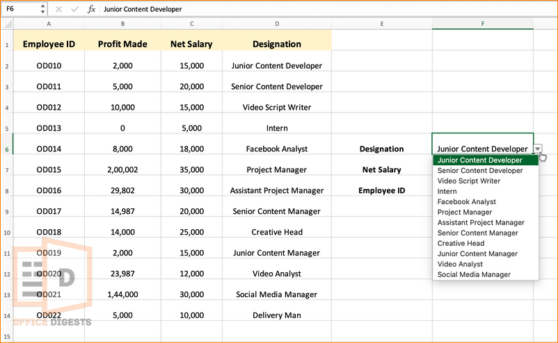
Explanation of the Data:

We have the Employee IDs, Net Salary, designation, b Profit Made columns. We also have a data validation list for the Designation Criteria and the Employee ID criteria.

Okay, so what are we up to?

We want to find out the Net Salary of that particular Designation. Alongside, we want to check the Employee ID and Profit Made by that Designator.

In short,

We want to look for values both Horizontally and Vertically. Apart from that, our dataset has the same array length.

So, all the three major points are checked. We are ready to proceed with the INDEX-MATCH Functions.

2. Launch The INDEX Function Followed By The MATCH Function

Okay, so let’s find out the Net Salary of the Employee in the F7 cell using the INDEX Function. Follow the steps along.

1. Click on the cell and type =INDEX function.
2. Select the array range. Remember, the array range is the range where the answer is present. The Formula should be like this: =INDEX(C2:C14,…)
3. Launch the MATCH Function since we want to return a row number to the INDEX function.
4. Set the Lookup_value for the MATCH function. In this case, the Designation drop down list is our lookup value. So, The Formula should be like this: =INDEX(C2:C14,MATCH(F6,…)
5. Determine the Lookup_array. The Lookup array should be the range where the MATCH function will search for the lookup_value.
6. Type 0 since we want an exact match.

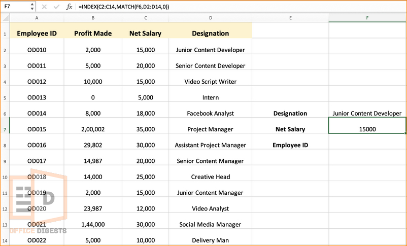
Final result: 15000 as the Net Salary.

3. Use The Column Number Argument For Multiple Criteria

For this scenario, we are going to elevate the problem a bit. We are going to add a dynamic list in the dataset so that Excel will return the value of the INDEX function accordingly.

For that, we will be using the MATCH Function twice. One for Row and the other for a column.

Remember, the array length and width of both INDEX and MATCH functions should be in sync.

So, let’s move on to the steps.

Our data validation list has two criteria. One is the Employee ID, and the other is the Profit Made criteria. So, we are going to extend our map.

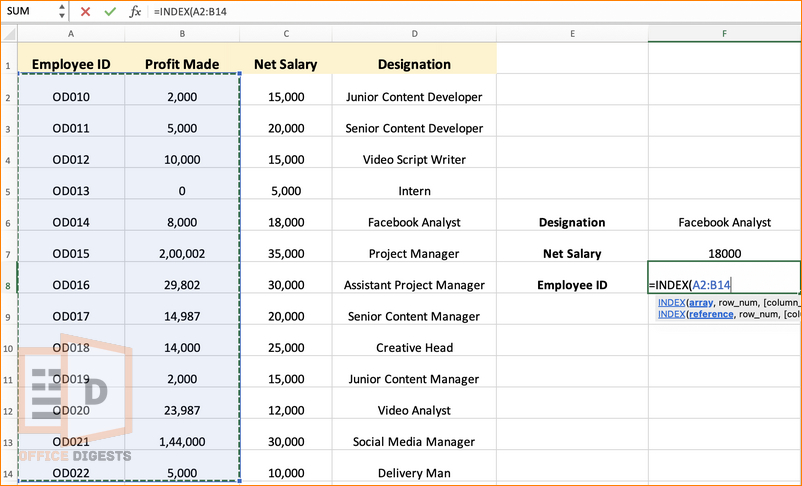
Follow the steps below to use INDEX and MATCH Functions both Vertically and Horizontally:

Launch the INDEX function and select the array length. This time, we selected two columns as our array. Both the columns had equal lengths.

Now, we used the MATCH Function to return a value from the rows. We selected the Designation as the lookup value and the designation range as the lookup_array. And to find the exact match, we selected 0.

Normally, this was enough.

But since we want to dynamically change the value depending on the validation list, we are entering the MATCH function again to return a value from the column this time.

Now, the lookup value is the E8 cell. Because we want to look for the value that will be constantly changing from the column headers.

Determine the lookup array. This time it will be the headers. Notice that the length and width of the array are equal.

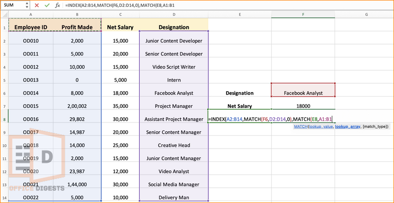
Finally, set the value to 0 as we are finding the exact match and Press Enter.

Final Result: OD014 as the Employee ID and 8000 as Profit Made.

Conclusion

In this post, we covered how the INDEX and MATCH function works and how you can use them combinedly to solve all the complex Lookup problems.

For practice, you should use the INDEX-MATCH even if the VLOOKUP function will work. In this way, you can set yourself apart in terms of skill.