Monthly Compound Interest Formula Excel Template |3 Examples

There are many banking, non-governmental organizations, and other financial institutions available out there that need to calculate this interest.

And to help them, there is Excel with so many features available that the possibilities are limitless in how they can calculate the interest using formulas and functions swiftly and efficiently.

In this post, we are going to teach you how to calculate the monthly compound interest formula in Microsoft Excel using a variety of formulas, accompanied by several visual examples.

You can use it as a template by changing it according to your needs.

What is the Monthly Compound Interest Formula?

Before we start with the main topic, you should first learn about what is the monthly compound interest and what is its formula.

Suppose you have loaned some money from a bank. When you borrow a given amount of cash for a specified amount of time, you must have paid some extra money in addition to the borrowed money.

That additional money paid at a set rate is known as interest. I guess you already know that. But do you know the compound interest formula?

Compound interest is calculated by adding the interest that had already accrued to the interest that was owed on the main balance. It’s the sum of the interest accrued on the original principal plus the interest accrued on the interest.

As the name implies, monthly compound interest occurs every month throughout the year. It’s quicker than basic interest since it’s calculated on top of previous interest calculations.

Now then, in order to calculate the compound interest on a monthly basis, use the following formula:

Basic Mathematical Formula:

In this formula, we can see that:

I = Monthly Compound Interest

P = Principal Amount.

R = Interest rate in percentage per year.

N = time in years.

Mathematical Example:

Imagine someone taking a $5000 loan with a 10% annual interest rate which will be ongoing for the next 5 years. Now, if you want to know what the monthly compound interest will be, you have to follow the below formula:

=5000 (1 + 10%/12)^12*1 – 5000

=$523.57

3 Monthly Compound Interest Calculation Formula in Excel

Now it’s time to understand how to calculate Monthly Compound Interest in Excel.

Here are the formulas to calculate compound interests in Excel:

Formula 1: Manual Calculation in Excel

Who wants to go for complex methods when there is a basic, easy way to calculate Monthly Compound Interest in Excel?

With this approach, we will use Excel and a simple mathematical formula to compute compound interest on a monthly basis.

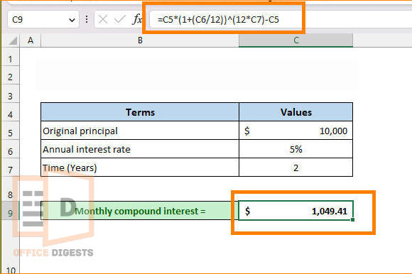
Let’s say a customer borrows $10,000 from a bank at 5% interest for two years. Now, let’s use the above formula to calculate compound interest on a monthly basis in Excel.

1. Open the spreadsheet file and choose a cell below your table. Our main principal/present value is located in cell C5. We need this value to be multiplied by the interest rate. So, on a blank cell, we will type: =C5*
2. When the interest is to be compounded monthly, we must divide the yearly interest rate by 12. So, enter the following formula: =C5*(1+(C6/12))
3. To account for the fact that interest will be compounded twelve times each year, we need to include a cell reference where the number of years is indicated. To reflect this, the formula inside the cell changes to =C5*(1+(C6/12))^(12*C7)
4. Deduct the original principal/present value, which is located in cell C5. So, all we have to do is to subtract cell C5. And our final formula becomes: =C5*(1+(C6/12))^(12*C7)-C5
5. Once you are done with all these steps, just hit the Enter button on your keyboard.

As you can see in the below picture, we correctly computed the monthly compound interest in MS Excel very easily.

Formula 2: Use The FV Function

Microsoft Excel includes the FV function, which belongs to the finance category, as a default feature. You can easily determine the potential return on investment with the help of this amazing function.

This FV function can be used in a variety of contexts. In this context, “payment” might mean either a single lump amount or a series of smaller, regular payments.

Here, however, we get the expected value of our investment back from the FV function.

Does the FV function seem new to you? Don’t know the syntax of this function? Take a look below:

In this syntax, we can see that:

• rate(required argument): The interest rate for each period is specified via the rate(required) parameter.
• nper (required argument): A number representing the total number of periods over which payments are made.
• pmt (optional argument): The pmt (non-mandatory) parameter sets the payment frequency in periods. If we want to avoid this argument, we’ll have to provide the PV argument.
• [pv](optional argument): The present value (PV) of the investment may be specified using the [pv] parameter. If not specified, it will be set to 0. It is imperative that we provide the Pmt argument if we skip it.
• [type] (optional argument): To specify when in the year the wages are generated, use the [type] input. If the salary is produced at the end of the period, it will be zero, and if it is created at the beginning of the period, it will be one.

Now that you know the syntax of this formula, it’s time for you to do what I say and continue reading the instructions below:

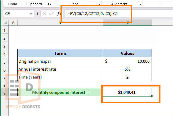
1. Open up your spreadsheet file and choose a cell below your table. We must first enter a rate into the FV function. I converted the annual percentage rate to a monthly rate by dividing it by 12. That’s why, in Cell C9, enter =FV(C6/12).
2. So that we may later define the total periods, I have multiplied the time in years (C7) by 12 to get the total number of months. To do that, enter =FV(C6/12,C7*12)
3. There will be no increase to the principal value over the investing term, therefore, the ‘pmt’ field will read “0.” To reflect this, the formula inside the cell should change to =FV(C6/12,C7*12,0,).
4. Then, because we are investing $100,000 as the initial capital and have skipped providing a value for “pmt,” I will refer to Cell C5 and indicate a negative PV. As a result, the formula is =FV(C6/12,C7*12,0,-C5).
5. At last, we may calculate interest by deducting the initial principal from the future value. Finally, the formula is as follows: =FV(C6/12,C7*12,0,-C5)-C5
6. After you’re finished, hit Enter to see the end result.

Formula 3: Apply the FVSCHEDULE Function

In the previous step, we saw how to determine the future value of an investment with a constant or stable interest rate using the FV (Future Value) function.

Now in this part, we are going to use the FVSCHEDULE function to Calculate Monthly Compound Interest in MS Excel.

This function calculates the future value of a payment, loan, or asset as interest rates change. Variable interest rates are rather prevalent in the real world due to inflation and other factors. In some cases, this technique is useful for knowing the future value of a current asset.

Now then, let’s take a look at the syntax of this FVSCHEDULE Function:

Here, in this syntax, we can see that:

Principal (mandatory argument): This argument means the present value of the investment.

Schedule (required argument): The numbers specifying how much interest will be added to the initial investment at regular intervals.

Pretty easy-looking formula, isn’t it? Now that you have successfully grasped the function, let’s implement this in our spreadsheet; what do you say?

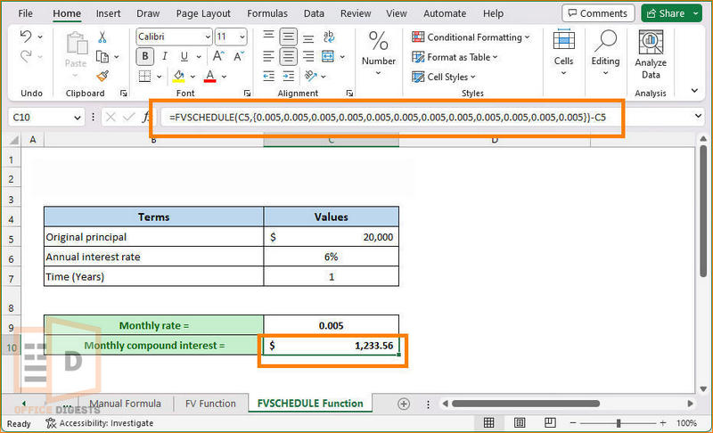
1. Open up your spreadsheet file and choose a cell below your table. To get started, we will have to enter the present value, which is located at cell C5 inside the FVSCHEDULE function. To do that, type the following formula in cell C10: =FVSCHEDULE(C5,…
2. The interest rate table is now presented as an array, which needs special attention. There are 12 months in a year, so I multiplied the yearly rate by 12 and entered the result in Cell C9 by entering this formula: C6/12
3. You are mistaken if you thought things were pretty easy! Now, enter this value 12 times acting as an array in the FVSCHEDULE formula, which will look like this: =FVSCHEDULE(C5,{0.005,0.005,0.005,0.005,0.005,0.005,0.005,0.005,0.005,0.005,0.005,0.005}).
4. Now it’s time the deduct the original principal/present value located at cell C5. Once you are done, the final formula will look like this: =FVSCHEDULE(C5,{0.005,0.005,0.005,0.005,0.005,0.005,0.005,0.005,0.005,0.005,0.005,0.005})-C5
5. Please press the Enter key now to see the result.

Now you have successfully calculated the Monthly Compound Interest by using the FVSCHEDULE Function.

Conclusion

There are three ways to calculate the compound interest in Excel. However, I suggest using the FV function more often. The function carries easy arguments compared to the FVSCHEDULE one.