
I bet almost everyone had their first thought – “Will the gridlines be visible during printing from an Excel workbook?” at least once in their lifetime.
During printing, it’s obvious that you want to get rid of all the gridlines in Excel. Even if you are creating a workbook, removing gridlines is a must.
Don’t know how to do it?
Keep Reading, As in this post, I will show you how to remove gridlines in Excel the easiest way.

About Grid Lines in Excel
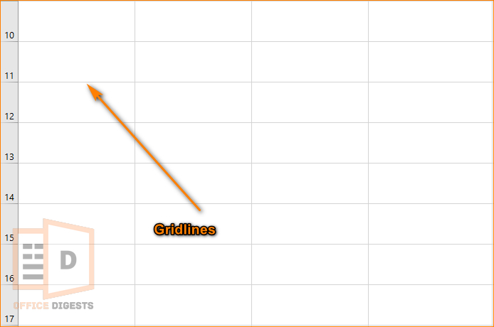
Gridlines are the faint lines that appear around cells in an Excel worksheet. They are meant to help you visualize and align data in a worksheet.
By Default, the color of the faint lines is black, which is set by Excel. Additionally, these faint lines are set across the whole worksheet. You cannot apply these lines to a specific cell or range of cells.
If you are a mobile photographer, you are well aware of grid lines. These lines help to align the subject so that you don’t take any zigzag images.
Similarly, grid lines help to define a cell, so that the text doesn’t overflow while you are typing.
In short, it separates two cells.
Three Hidden Facts About Gridlines
Did you know you can do some really cool stuff with these fainted lines?
Here are three hidden facts:
1. You can change the color of gridlines
By default, gridlines in Excel are light gray. However, you can change the color of these grids to any color you like.
Simply right-click on a cell. Select Format Cells option and then click on the Border tab. From there, you can select the color you want for your grids.
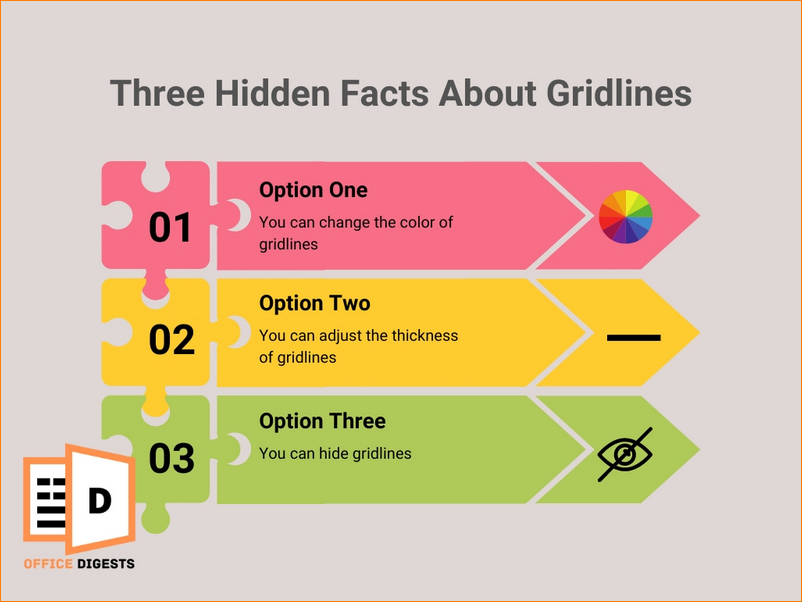
2. You can adjust the thickness of gridlines
In addition to changing the color of gridlines, you can also adjust the thickness of the lines.
To change the thickness of the border, go to the Home tab on the ribbon, and then click on the Format button in the “Cells” section. From there, select Border and then choose the thickness you want for your grid lines.
3. You can hide gridlines
While gridlines are helpful for aligning data, they can also be distracting when you want to focus on the content of a worksheet.
You can easily hide gridlines by going to the View tab on the ribbon, and then unchecking the Grid lines box. This will make the grid disappear, but they will still print when you print the worksheet.
How To Remove Gridlines in Excel Worksheets
By default, the faint lines are visible in Excel. There are multiple ways to remove grids. You can fill a range of cells with a white color. Or you can follow the method down below.
Here are the steps to remove grid lines in Excel worksheets:
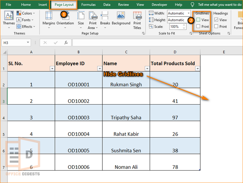
- Go to the Page Layout Tab in the ribbon bar.
- Uncheck the View checkbox under the Gridlines option.
Easy as it seems.
However, you should keep some important points in mind.
Point No.1
Unchecking the View checkbox under the Gridlines option will only hide gridlines on the active worksheet.
To hide gridlines on multiple worksheets, you have to select the worksheets altogether by pressing the Control button (for Windows) and the Cmd Button (for mac users). Then you have to Uncheck the View checkbox option.
Point No.2
You can use the fill background to make the entire worksheet white. This will remove all the grid lines from Excel.
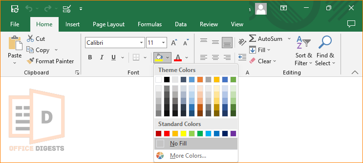
Press Ctrl+A to select the entire worksheet. Go to the Home Tab and select the Fill Color. Set the fill color to white.
Point No. 3
By default, grids are not printed. To show gridlines in Excel when printing, click on the checkbox that says “Print”, under the Gridlines option within the Page Layout tab.
We will share more detailed information about printing grids in Excel.
How to Remove gridlines in Excel when Printing
By default, during printing a worksheet in pdf, the grids are invisible, making it user-friendly. However, in some cases, due to technical glitches, you may end up ruining your file.
Don’t worry.
Go to the Page Layout Tab and on the rightmost side there is an option called Gridlines. Under that option, there are two more options (view & print). If you want to remove the grids, make sure to uncheck the print checkbox. After that, go to the print view mode and check whether the lines were removed or not.
Missing Gridlines in Excel When Printing?
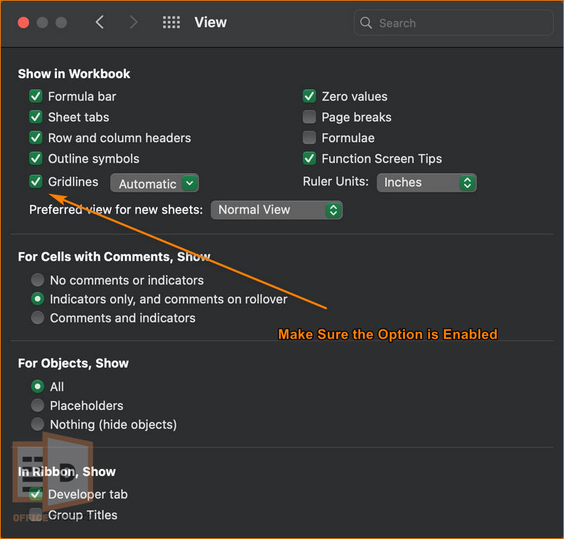
If you are unable to find the Grid lines option in the page layout tab, you have to ensure that the option is enabled in the worksheet.
For Mac Users
Go to Excel > Preferences > View > Checkmark the Gridlines option and set the color to Automatic or any color you want.
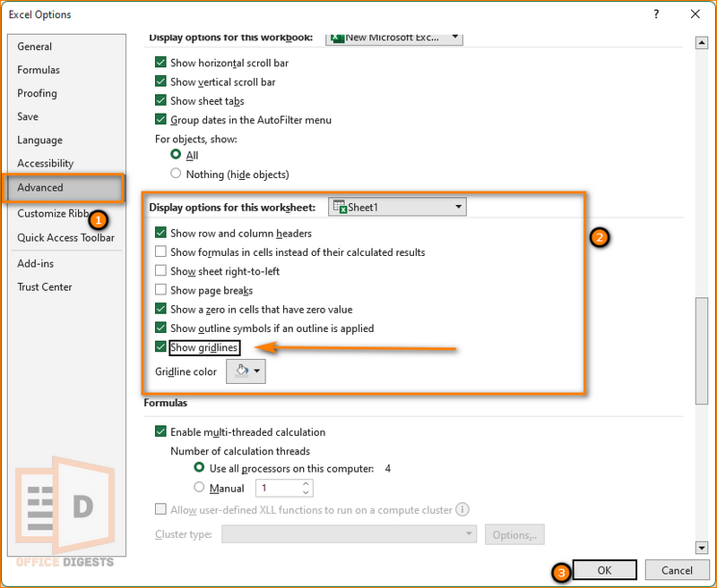
For Windows Users
Go to File > Options > Advanced Options > Display For This Workbook > Ensure that the Gridline checkbox is enabled. Then go to the Page Layout option to show or hide gridlines in Excel.
How To Remove gridlines in Excel Graph
If you are more into graphs like me, then this section is the suitable tutorial for you.
Whenever you create a graph, there are grid markers, which are annoying most of the time.
We want our graphs to look neat and clean. We always like to combine two graphs in Excel for a sleek look. And so, removing the lines is a necessary deal.
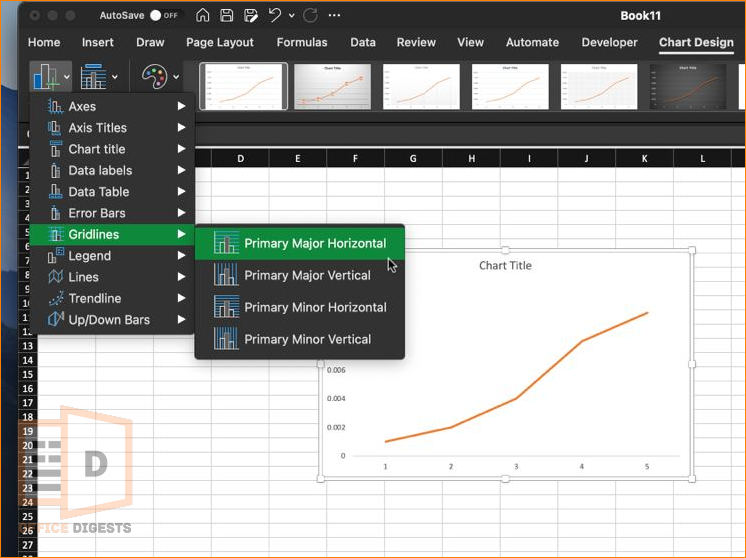
Select the chart you made and click on Chart Design from the Ribbon bar. Select “Add Chart Elements” and navigate to Gridlines. By default it is set to “Primary Major Horizontal”. Click on it and the grids will disappear.
Now, if you want to add lines for specific cells, then move to the next section.
How to Add Gridlines in Excel for Specific Cells
Actually, there aren’t any direct ways to add a grid line to a specific cell. You can perform this procedure by manually filling the unnecessary cells with white filled color.
This will only show gridlines to necessary parts of your dataset.
However, there’s another way which is adding borders to cells.
First, select the whole worksheet and remove the grids. Then select the necessary range of cells and go to the Home Tab. Under the Font section, you will see a border icon. Click on the drop-down menu and select All borders. This will apply borders to the cell lines.
FAQ
Q: How to change the color of gridlines in Excel?
A: For Macintosh users, Select Excel > Preference > View > Gridlines (Automatic) > Change the color as your preference. If you are a Windows user, go to File > Options > Advanced Options > Display For This Workbook > Gridlines > Change Gridline color.
Q: How to make gridlines darker in Excel?
A: You can make borders darker by changing the depth of the border to a few millimeters. However, you cannot make the gridlines darker or deeper.
Conclusion
Removing the grid lines is necessary while printing. In most offices and high schools, they provide low performance grades if you print your Excel file with grids.
That’s where our post comes in handy. With all the easy steps mentioned in this post, you can easily deal with hiding the faint lines.

