It is common to come across situations in which we must sum a range of values over multiple columns. In this tutorial, we will show you how to SUMIF multiple columns by applying functions such as SUM, SUMIF, SUMIFS, and also the mixture of SUMPRODUCT, ISNUMBER, and SEARCH functions.
Excel, as we all know, has an extensive set of functions that can be used to execute a wide variety of equations with data. It is possible that those who are experienced with the SUMIF function may believe that changing it to SUMIFS is as simple as adding an extra S and meeting a few more conditions. On the surface, this seems to be perfectly logical. However, when it comes to Microsoft, logic is not necessarily the case.
In this article, we are going to show you the syntax of the SUMIFS function and how to SUMIFS multiple columns.
5 Easy Ways to SUMIFS Multiple Columns
Now let’s take a look at some of the best 6 easy ways to SUMIFS multiple columns.
1. By Using the SUMIFS Function
In the very first method, we are going to show you the easy method of doing this job, which is the SUMIFS function. But first, let’s take a look at the plain syntax of the SUMIFS function:
=SUMIFS (sum_range, criteria_range1, criteria1, [range2], [criteria2], …)
Now for the explanation of each section of the syntax, take a look at the below part:
- sum_range: This section specifies the range across which we wish to sum.
- criteria_range1: specifies the range within which the criteria are located.
- Criteria 1: Specify the criterion we are looking for in the criteria range1.
Because of the structure of the SUMIFS function, it will only sum one column based on criteria that are available in several columns at any time. To Sumif the sum range of many columns is large, we must add a helper column to the equation.
So, in the first step, we will have to add a helper in the column as a Subtotal adjacent to the range. To do that, follow the steps below carefully:
- Open the spreadsheet in Excel and enter the following formula given below in cell I7: =SUM(C7:H7)
- Hit the Enter button on your keyboard and drag it down all the way to cell I27. And in a minute, you will see the remaining subtotal appears.
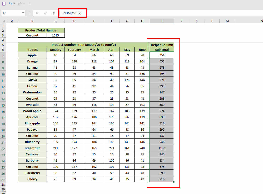
- Now fill in any empty cells with the given formula. (We chose the C3 cell, as you can see in the screenshot below): =SUMIFS(I7:I27,B7:B27,B3)
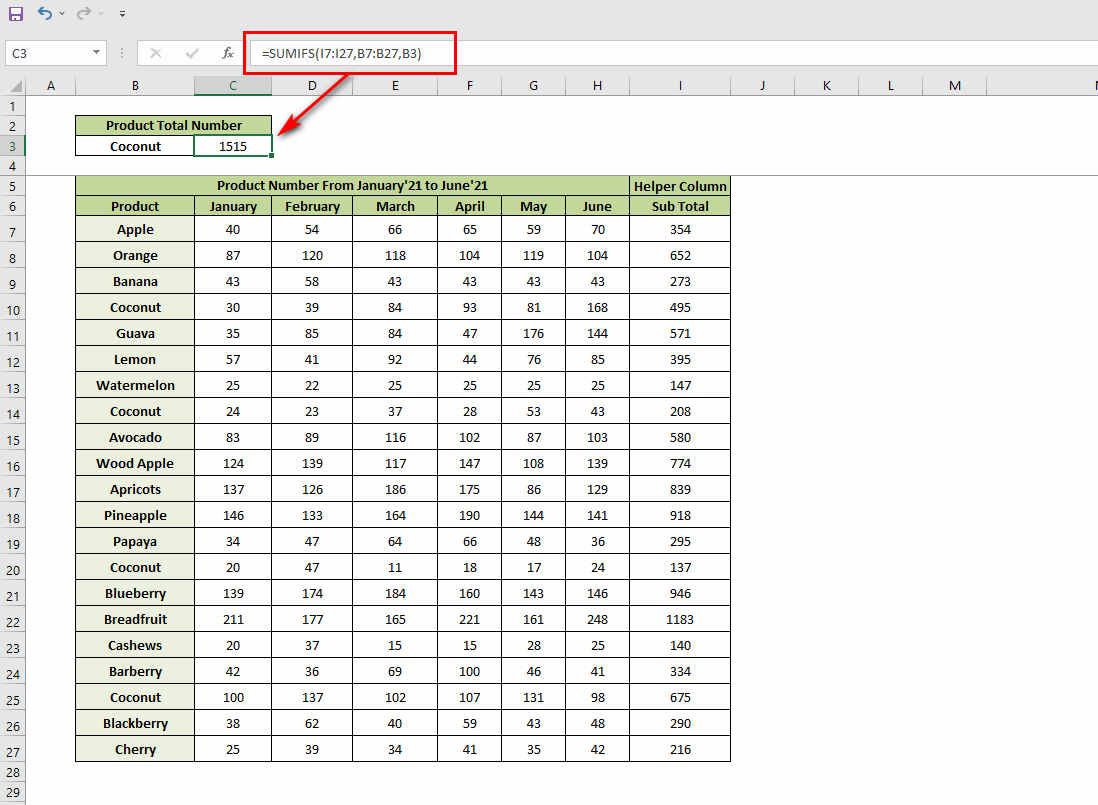
Once you are done filling the C3 cell with the formula, you will immediately see the product total sale number, which is in cell B3. For example, we wanted to see the total sale number of Coconut. So, we typed Coconut in cell B3, and in C3, we got the total sale number.
Now, let’s see the explanation of the formula.
Detailed Explanation of the Formula:
- I7:I27: This is the total sum range.
- B7:B27: It is the criteria range 1.
- B3: This is the criteria that we want to see.
2. By Using the SUM Function
Now we will use the SUM function. It’s quite similar to the previous one, but still, similarities don’t affect the formula. There are some major changes here. However, now let’s take a look at the syntax of the SUM function:
=SUM(number1, [number2],…)
And so, we must change the SUM function into an array function in order to complete the task. To do that, follow the below step carefully to Sumifs multiple columns:
- Open the spreadsheet and enter the below-given formula into any cell (we chose C3, as you can see in the screenshot below): =SUM((C7:C27+D7:D27+E7:E27+F7:F27+G7:G27+H7:H27)*(–(B7:B27=B3)))
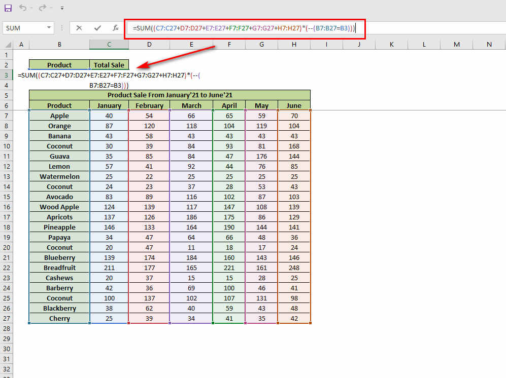
- After entering the formula, press CTRL+SHIFT+ENTER simultaneously because it is an array function.
Now, the total sale number of coconuts will appear in cell C3. Although, if you want to count the total number of product sales, you may enter any name for the item in the B3 field.
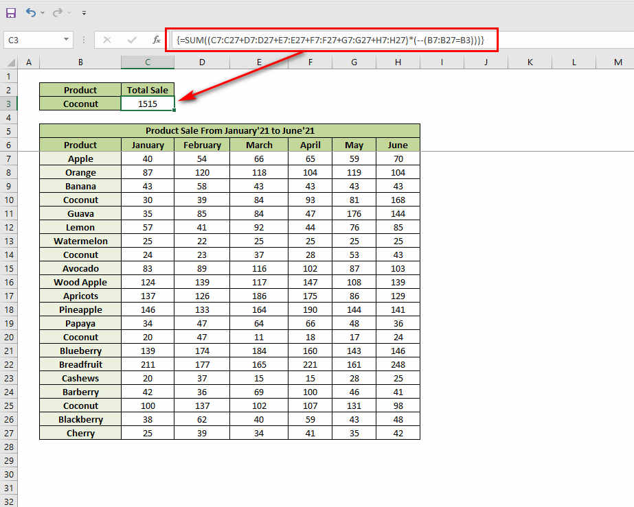
In this formula, we can see-
The part (C7:C27+D7:D27+E7:E27+F7:F27+G7:G27+H7:H27) specifies the sum total of the six ranges.
(B7:B27=B3) this part is the range value (cell B3) from which we will get the total sale number.
3. By Using the SUMIF Function
According to what we learned before, the SUMIF function doesn’t really enable us to sum ranges from many columns at the same time. However, we may make use of a helper column to do what we need. The SUMIF function has the following syntax:
SUMIF(range, criteria, [sum_range])
In this syntax of the formula, we can see:
- range: specifies the cells in which the criteria are to be found.
- Criteria: a condition that will be applied in the range is defined by criteria.
- [sum_range]: specifies the range of values that we wish to show.
Now, let’s move on to the main procedures of how to Sumifs multiple columns by using the SUMIF function. But first, we will have to make a helper column in column I, just like we did in method 1. Follow the below steps to do that:
- Open the spreadsheet in Excel and enter the following formula given below in cell I7: =SUM(C7:H7)
- Hit the Enter button on your keyboard and drag it down all the way to cell I27. And in a minute, you will see the remaining subtotal appears.
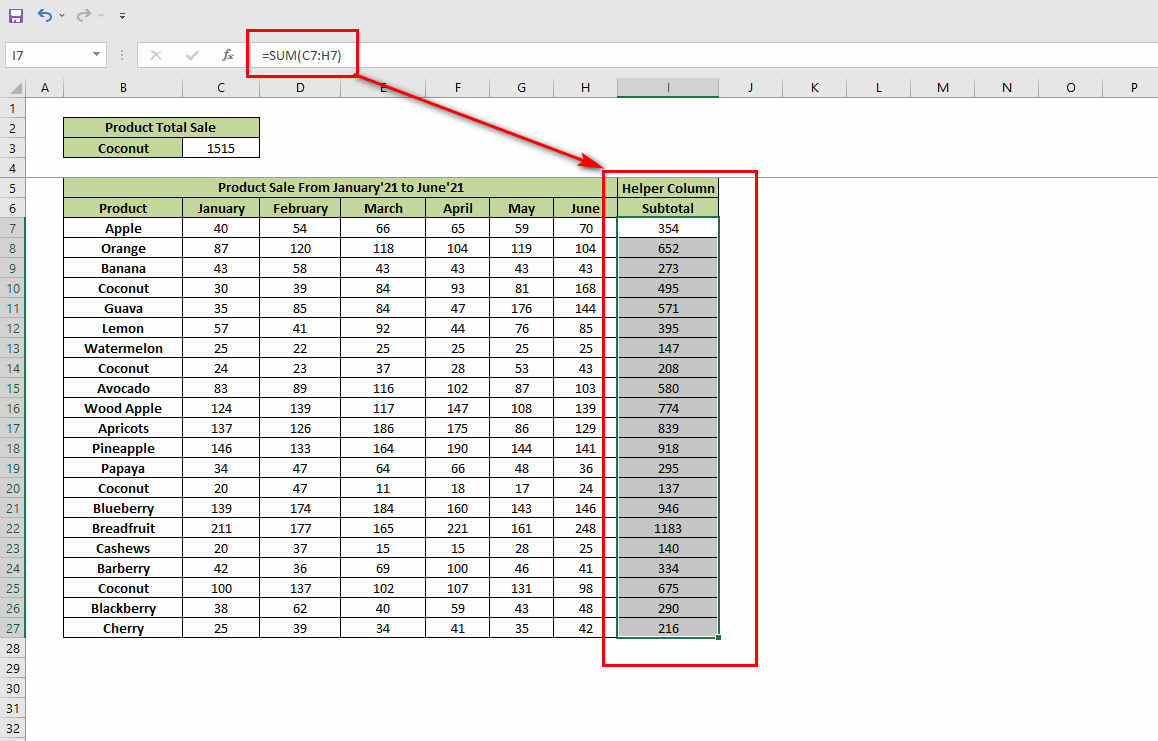
Now, type the following formula in cell C3:
=SUMIF(B7:B27,B3,I7:I27)
In this formula, we can see:
B7:B27 is the range of the data.
B3 is the criteria.
And I7:I27 is the sum range of this table.
Now, after entering the formula in cell C3, press the Enter button on your keyboard, and the total sale number of cell B3 (Coconut) will appear instantly in cell B3.
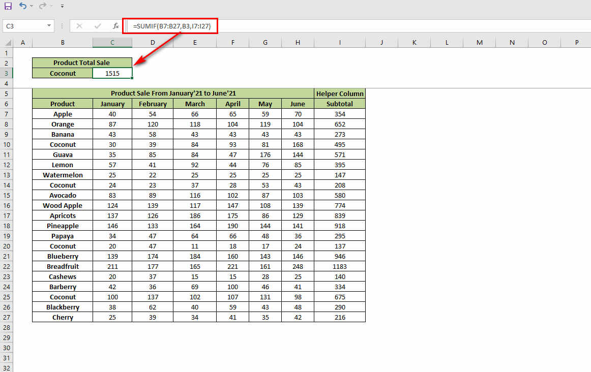
So, in this way, you can actually Sumifs multiple columns in Excel by using the SUMIF function.
4. By Using the SUM SUMIF Function
The SUMIF function may also be used to sum several ranges at the same time, which is described below. This may seem like a lot of effort, but if you just do have some columns to process, it is doable. The SUMIF function, which we learned about in Method 3, must be applied to every single column, and the conditions must be applied to each column.
Consider the following scenario: we wish to total the product sales in several months, for example, January, April, and June.
So, to do that, follow the steps below:
- Open the spreadsheet and enter the formula given below in cell C3: =SUMIF(B7:B27,B3,C7:C27)+SUMIF(B7:B27,B3,F7:F27)+SUMIF(B7:B27,B3,H7:H27)
- Press Enter, and you are done. The total sale number of coconuts in the months of January, April, and June will appear instantly.
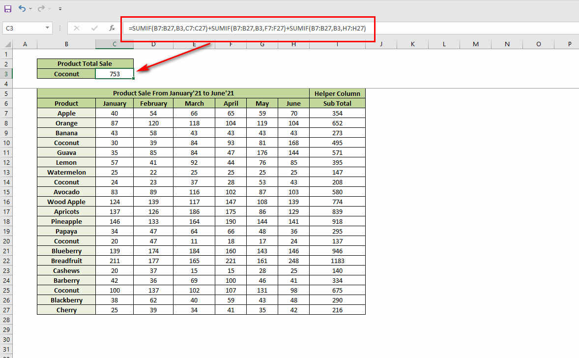
In this formula, we can see:
SUMIF(B7:B27,B3,C7:C27): is a total of product sales for B3 products in the B7:B27 range, with the total coming value of the C7:C27 range being sent to the sum.
The remaining the other sections serve the same job as the first.
And in this way, this formula works.
5. By Using the SUMPRODUCT Function
SUMPRODUCT function can also be used to get the total of a particular product.
The plain syntax of the SUMPRODUCT function is:
=SUMPRODUCT((criteria_rng=”text”)*(sum_range))
Because we are interested in the overall number of sales of a certain product, we may use the product name as a text reference, as you can see in the syntax above. And the code will return the amount from the sum range.
Now, follow the below steps to get the total sale value:
- Open the spreadsheet and enter the below formula in cell B3: =SUMPRODUCT((B7:B27=”Coconut”)*(C7:H27))
- Press Enter, and you are done. The total sale number of coconuts will appear instantly.
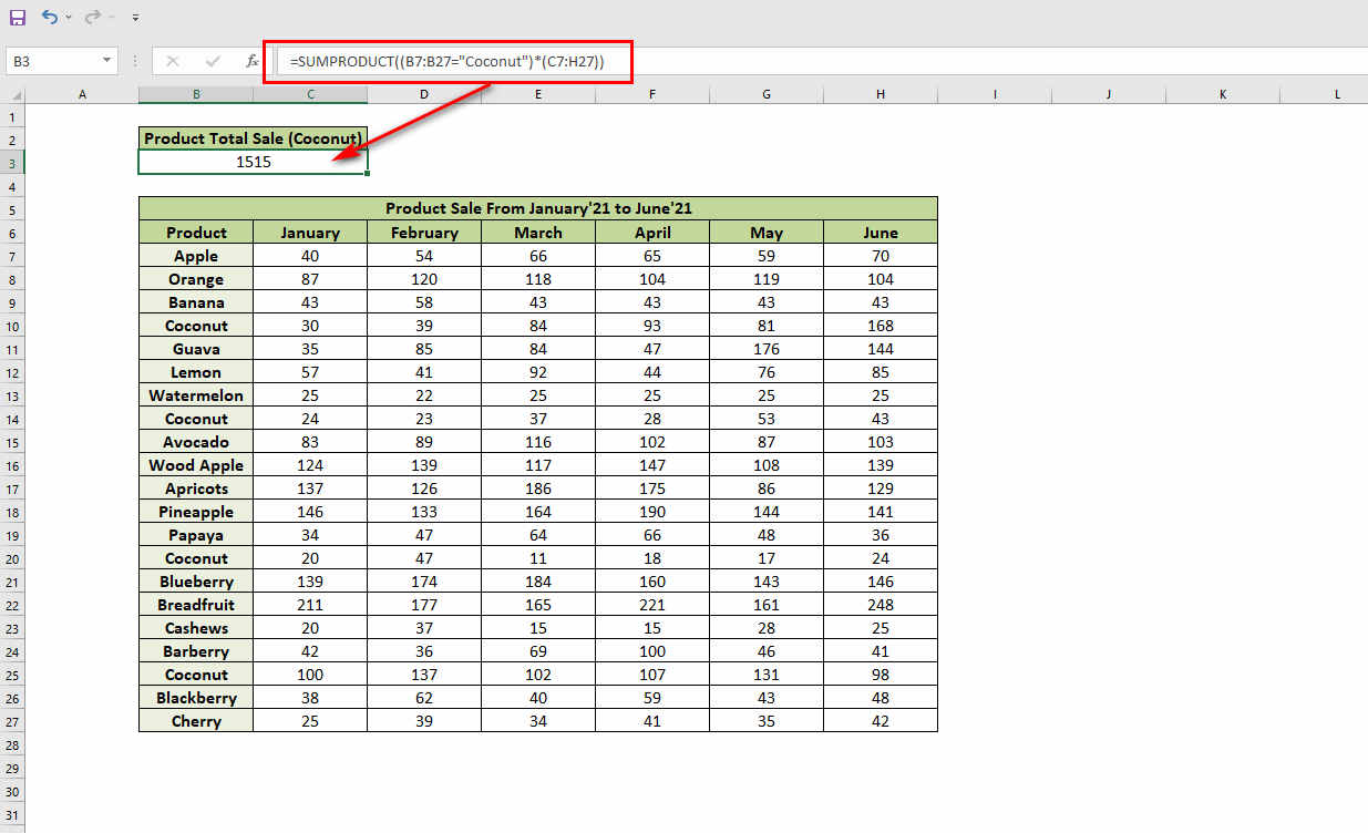
In the formula, we can see:
(C7:H27) produces a True or False value depending on the criteria.
(B7:B27=”Bean”)*(C7:H27) multiply the values by the criteria that determine whether they are True or False.
And at the end of the day,
SUMPRODUCT((B7:B27=”Bean”)*(C7:H27)) returns the total amount of money that was sold.
And in this way, you can easily Sumifs multiple columns by using the SUMPRODUCT function.
Conclusion
The summation of a range of values in several columns can easily be done using the SUMIF and SUMIFS functions, which have minor tweaks in the formulae though. Also, after we provide certain criteria in the calculation, the SUMPRODUCT function does the task with simplicity. We hope you find the ways mentioned above on how to Sumifs multiple columns to be understandable and easy to follow.


