If the VLOOKUP function in Excel is used to search up one or more values, it will only return the first match and will not return any more matches. As we already know, the VLOOKUP function is intended to return just the value corresponding to the first occurrence of a lookup value found in a column that has been specified by the users.
But what happens if a lookup value has several matches inside a certain range of values? Or, for whatever reasons, you want to return all matches found in a range. Worry not; there are a number of different approaches to using VLOOKUP, also known as vertical lookup, in Microsoft Excel to retrieve data based on a number of matches.
In this article, we are going to demonstrate how to deal with Vlookup and return all matches.
So, stick with this article until the end to learn more.
6 Easy Ways to Use Vlookup and Return All Matches in Excel
The Vlookup formula searches for a certain value in the leftmost column of the table and returns a value from that same column, in the same row, based on that search. This method, on the other hand, is unable to retrieve data from a column based on multiple matches. This means that in order to do a value lookup and get all matches in a column, we need to include additional functions and formulae.
Here are the steps to use VLOOKUP to return multiple matches in Excel:
1. Use Vlookup to Return All Matches in a Column
In this first method, we are going to use the Vlookup function to return all the matches in a column. As you can see, the below image that shows a table with the names of various individuals and the departments in which they work, all selected at random. Assume that we want to display the names of all of the workers who are employed in the Plan department in a separate column.
So, to do that, we need to do some tricks with the formula. Follow the below steps carefully to understand what we did to return all matches:
- Open the Spreadsheet in Excel and select cell C14.
- Type the following formula into the cell and hit the Enter button on your keyboard: =INDEX($C$3:$C$11, SMALL(IF(($C$13=$B$3:$B$11), MATCH(ROW($B$3:$B$11), ROW($B$3:$B$11)), “”),ROWS($A$1:A1)))
- Press the Enter button, you will see the name of the employee of the Plan department in cell C14.
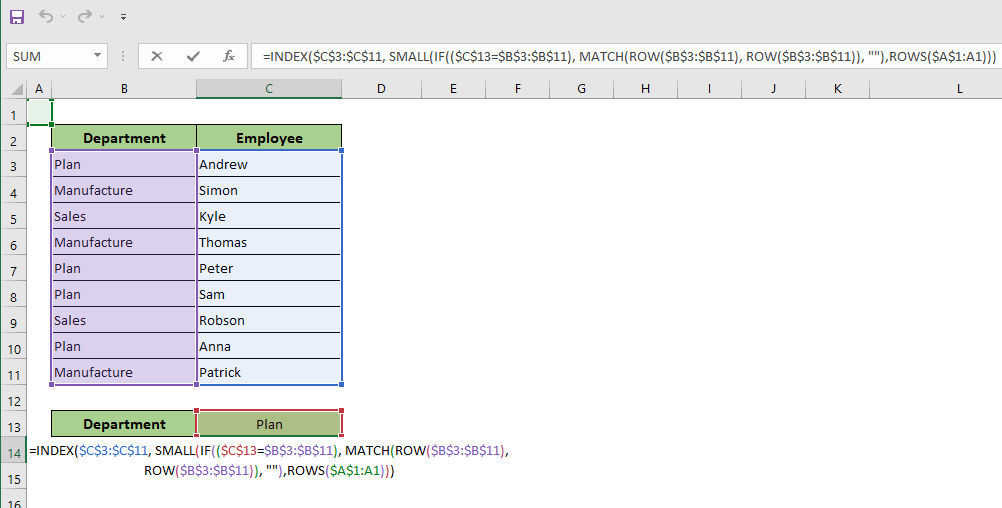
- Copy and paste that formula downward by using the fill handle option, which is located in the right bottom corner (the plus icon).
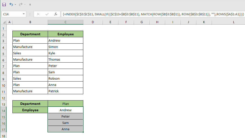
Now you will get all of the names of the Plan department from cell C14 to cell C17 at once.
Detailed Explanation of the Formula:
The formula works in different sections. Below we explained the formula separately:
- $B$3:$B$11: Evaluating through the provided cell references, the ROW function retrieves the row values and produces the following array: {5;6;7;8;9;10;11;12;13}
- MATCH(ROW($B$3:$B$11), ROW($B$3:$B$11)): The MATCH function, in this case, changes the collected row numbers beginning from 1 to a different format. In other words, this section of the algorithm gives an array of the numbers: {1;2;3;4;5;6;7;8;9}.
- IF(($C$13=$B$3:$B$11), MATCH(ROW($B$3:$B$11), ROW($B$3:$B$11)), “”): This section of the equation, which makes use of the IF function, yields the index value of the rows that match the provided criteria. As a result, this section yields an array of: {“”;2;””;4;””;””;””;””;9}.
- SMALL: This formula includes the SMALL function, which extracts the very first small number discovered in the preceding step and gives that value to the INDEX function’s second parameter (row number).
- Index: Lastly, the INDEX function displays the name of the employee depending on the row number that has been given.
- ROWS: When the SMALL function is used in this calculation, the ROWS function is used to specify the K-th value. When filling in the remaining cells with the Fill Handle method, the formula extracts data from the K-th cell using the SMALL function, which is then used to take care of the rest of the cells.
In this way, this IndexMatch function combo works. But if you are using the Office 365 application, then you can also use the FILTER function instead of the Index Match function combo to return all the matches at once.
In case of using the FILTER function, follow the below steps to do the task:
- Open the Spreadsheet in Excel and select cell C14.
- Type the following formula into the cell and hit the Enter button on your keyboard: =FILTER(C3:C11,C13=B3:B11)
- Press the Enter button, you will see the name of the employee of the Plan department in cell C14.
- Copy and paste that formula downward by using the fill handle option, which is located in the right bottom corner (the plus icon).
Now you will get all of the names of the Plan department from cell C14 to cell C17 at once.
2. Use Vlookup to Get All Matches in a Row
Suppose you have a spreadsheet that requires you to return the matches horizontally. So, in that case, you won’t be able to use the previous method to do the job. But worry not. If you want to return all matches in a row, then follow the below steps carefully:
- Open the Spreadsheet in Excel and select cell C14.
- Type the following formula into the cell and hit the Enter button on your keyboard: =INDEX($C$3:$C$11, SMALL(IF($C$13=$B$3:$B$11, ROW($B$3:$B$11)-MIN(ROW($B$3:$B$11))+1, “”), COLUMNS($A$1:A1)))
- Press the Enter button, you will see the name of the employee of the Plan department in cell C14.
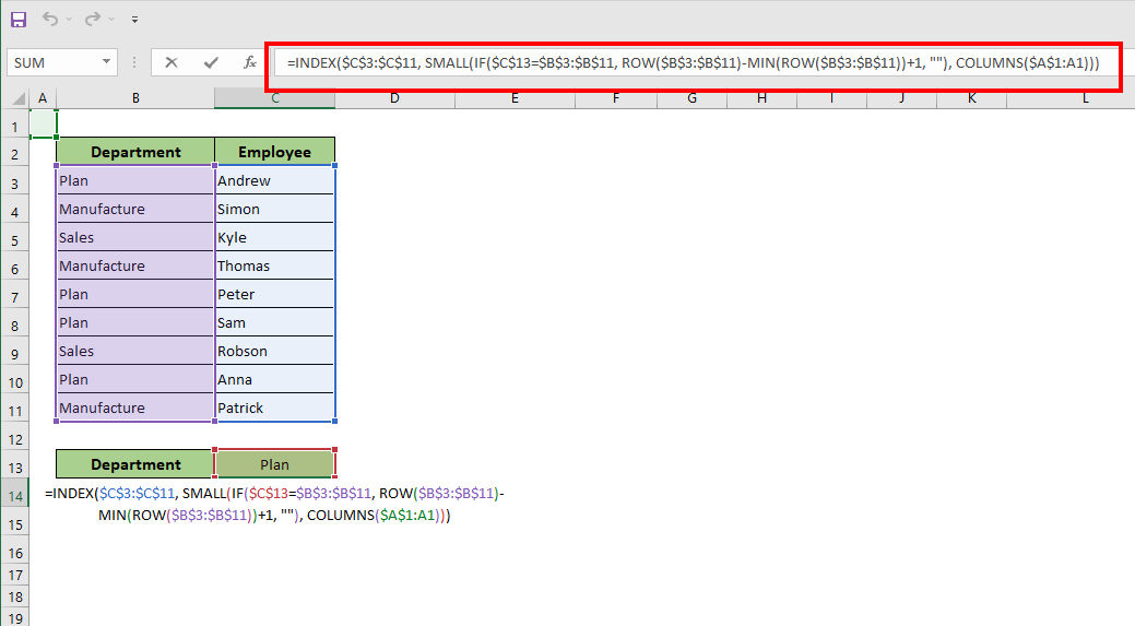
- Copy and paste that formula to the right by using the fill handle option, which is located in the right bottom corner (the plus icon).
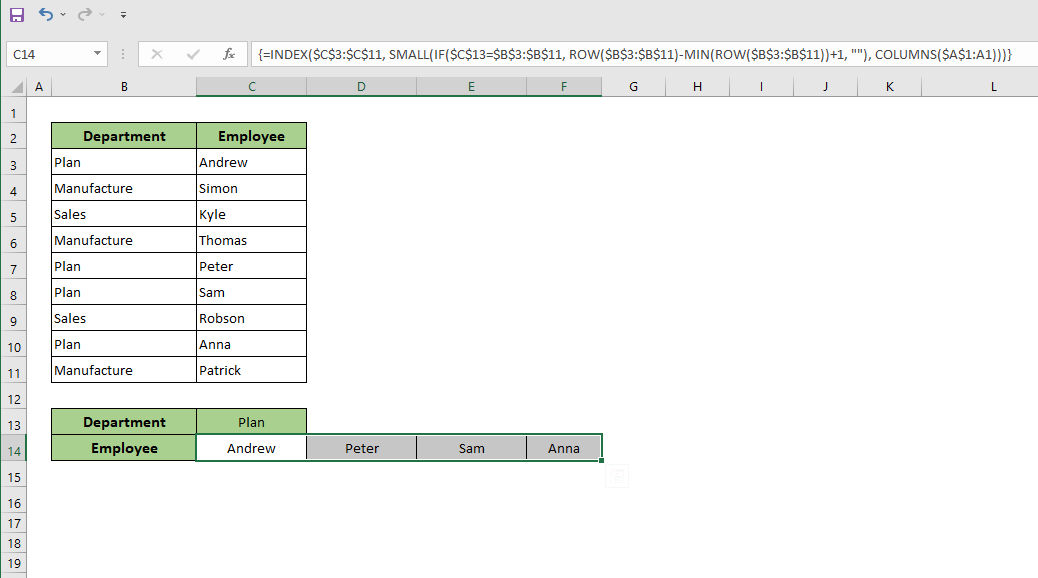
Now you will get all of the names of the Plan department from cell C14 to cell F14 at once.
Detailed Explanation of the Formula:
There are many similarities between the two long formulas used in the preceding method, where the output had to be shown vertically and the one used in this method. With the exception of the fact that we are specifying the sequence number of the SMALL function here, there aren’t many changes. To collect data from the fields while the formula is auto-filling them sideways, it will maintain the sequence number of the SMALL function.
Now, if you don’t use MS Excel, and are an Office 365 user, then you cant use the above formula. You have to use the FILTER function that we have given below. Enter the formula below in cell C14, and hit enter:
=TRANSPOSE(FILTER(C5:C13,C15=B5:B13))
In this method, you will have to You will need to integrate the FILTER function with the TRANSPOSE function in order to complete this procedure. In Excel, the TRANSPOSE function is used to transform a vertical range of cells into a horizontal range of cells or vice versa. Additionally, you have to be an Excel 365 user in order to make use of this combination formula.
3. Use Vlookup to Pull All Matches Based On Criteria
By following this method, you will be able to pull all matches based on criteria. To demonstrate this method to you, we have included one additional column in the center of the table. In this column, the project IDs are kept, which are then linked to the employees in Column D.
Suppose we would like to know the names of workers who are now engaged in the Plan department on project ID PB 320.
So, to do that, follow the below steps carefully:
- Open the Spreadsheet in Excel and select cell C17.
- Type the following formula into the cell and hit the Enter button on your keyboard: =IFERROR(INDEX($D$5:$D$13, SMALL(IF(1=((–($C$15=$B$5:$B$13)) * (–($C$16=$C$5:$C$13))), ROW($D$5:$D$13)-4,””), ROW()-16)),””)
- Press the Enter button, you will see the name of the employee of the Plan department on project ID PB 320 in cell C17.
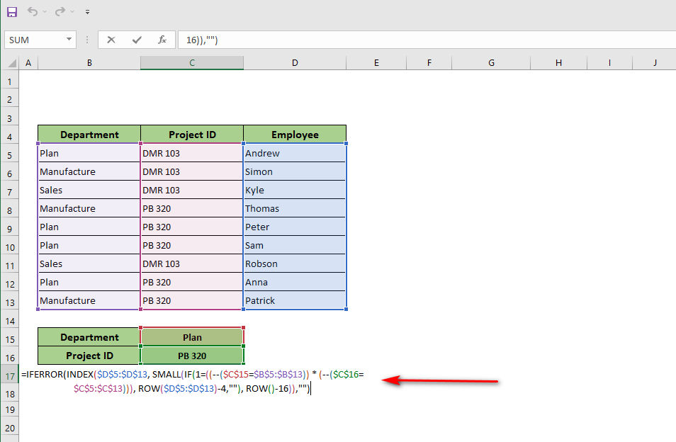
- Copy and paste that formula downwards by using the fill handle option, which is located in the right bottom corner (the plus icon).
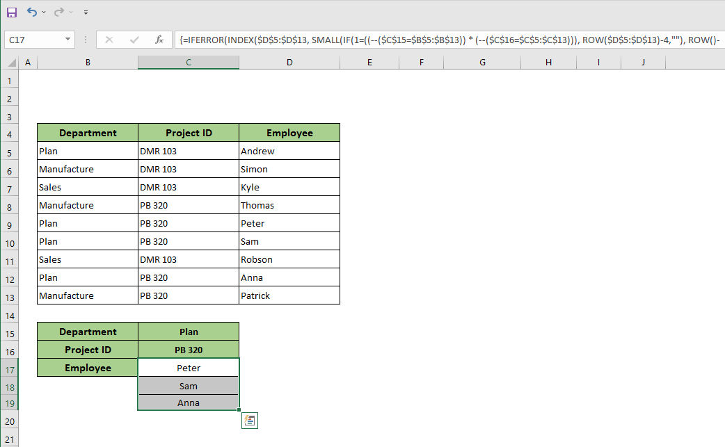
Now you will get all of the names of the Plan department from cell C17 to cell C19 at once.
Detailed Explanation of the Formula:
As usual, this formula is indeed very close to the one applied in the prior procedure. But still, there are some other features and steps that distinguish this formula. For instance:
- If an error is detected in this formulation, the IFERROR function is being used to display a personalized output. If no error is detected, the output is left as is.
- It is possible to integrate two separate conditions in this method, and the boolean numbers (TRUE or FALSE) are converted into one or zero with the assistance of the double-unary function. After that, the function will return the identification number of the rows that have been found to fit the specified criteria.
- ROW($D$5:$D$13)-4: The row position of the Employee heading is represented by the number ‘4’ in this section.
- ROW()-16: In this section, the numerical value “16” signifies the prior row number of the very first output cell, which was previously shown in the preceding section.
4. Use Vlookup to Extract All Matches with AutoFilter
If you are lazy like me and don’t like the hassle of using any formulas, then this AutoFiller method might be the perfect solution you are looking for because we can pull the data very simply if we use AutoFilter, which allows us to retrieve information based on all matches.
Now, for the purpose of extracting the names of workers from the Plan department, we must follow the procedures outlined below:
Part 1:
- Open the spreadsheet in Excel and select the whole data table, and right-click on the mouse.
- Go to the Filter option and select the option called Filter by Selected Cell’s Value.
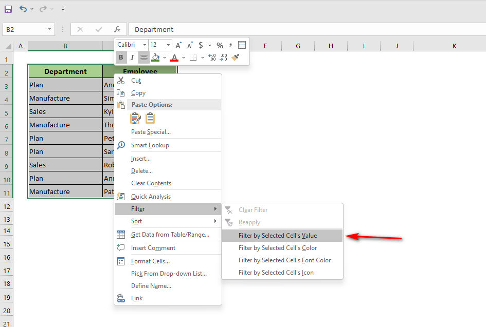
Once you are done completing all the steps above, you will see that the filter button on the header has now been activated. Now, follow part 2 below to extract all matches based on criteria.
Part 2:
- From the Department heading, choose the Filter button from the drop-down arrow.
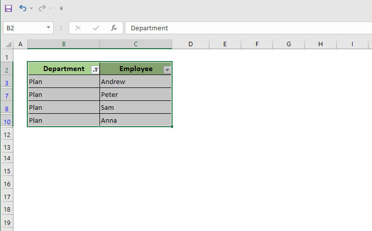
- Only choose the Plan option from the drop-down menu.
- Once you have clicked OK, you are finished.
Now, only the employee’s name of the Plan department will be filtered out. As you can see in the screenshot below:
5. Use Vlookup to Return All Matches with Advanced Filter
Just like the previous method, if you want to return all matches in an advanced way, then you can use this method. You may also make use of the Advanced Filter, which requires you to create the criteria by choosing the criterion range of your Excel spreadsheet before applying it. The criterion range shown in the below image is B14:B15.
Hence, follow the below steps to do that:
Part 1:
- Choose the whole data table by mouse.
- On the Data ribbon, under the Sort and Filter drop-down menu, choose the Advanced command from the list.
- A dialogue box titled Advanced Filter will now appear on the screen.
Part 2:
- On the Advanced Filter dialogue box for the List Range input, choose the whole data table from which to draw information.
- For the input of the Criteria Range, choose the values B14:B15.
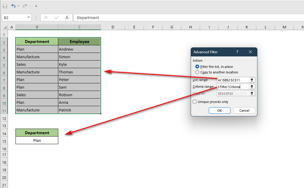
- Click on the OK Button.
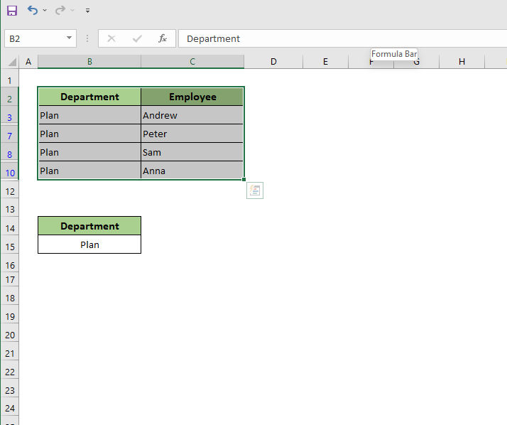
And now, voila! You will be presented with a filtered return that only includes the names of workers who work in the Plan department.
6. Use Vlookup to Return All Matches by Formatting as Table
Now, in this method, we are going to show you a simple method through which you can return all matches by formatting the data as a table.
To do that, follow the steps below:
Part 1:
- Open the spreadsheet and select the whole data range.
- Now, on the Home tab, from the Format as Table drop-down menu, select a table format that you like.
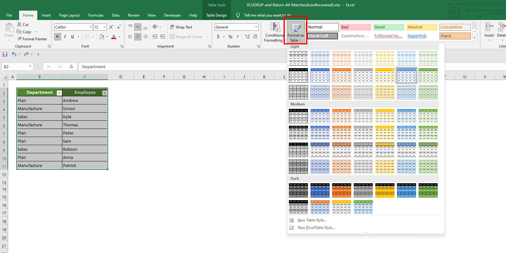
Once you have done that, the data range will become e table and have a filter drop-down arrow on the headers.
Part 2:
- Now, just like the previous methods, click on the filter arrow and select only the Plan option.
- Click on the OK button, and the process is done.
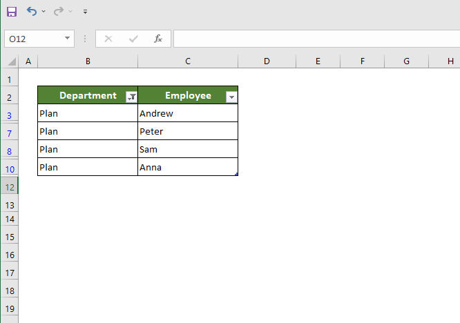
Now, as you can see in the screenshot above, the table will be filtered out, and you will only see the names of the plan departments.
Conclusion
Returning all matches by using VLOOKUP can be pretty tough if you don’t have the proper knowledge of different types of formulas. So, we rounded up some of the best ways to use Vlookup and return all matches in Excel. We hope this article has helped you to do the job.


